Introduction
This is the book I which I had when I made my transition from generalist Software Engineer to ML engineer at Deepmind.
I started it as interview preparation, but it quickly evolved into a more comprehensive list of skills I acquired during my time at Google Deepmind. A lot of the skills required in ML performance are scattered around in different resources, or have to be learnt on the job by talking to more experienced engineers. This book tries to assemble the most important bits in a single place.
I use Gemini extensively to refine my words (I am not a native english speaker) and to generate diagrams (with Nano Banana 3.)
Goals and Non-Goals
The book is an introduction to the most important concepts required to succeed in ML engineering. Its goal is to cover a large breadth of subjects but not to dive too deep into any single one. Most of the topics discussed are active research problems with new papers being published frequently. Building a T-shaped skillset - good knoweldge in a lot of subjects and expert knowledge in a handful of others - is often recommended for a successful career. Readers are encouraged to go and read the latest papers in the subjects that interested them the most.
Prerequisites
A good understanding of computer programming in Python is required. Linear algebra, Machine Learning, and distributed programming skills will greatly help understanding the material but are not necessary.
Structure
The book gradually introduces concepts that build on top of each other as the chapters go by. We first introduce the basic APIs that are commonly used to build ML models. After that, we have a small chapter discussing the backward pass and its performance implications. Then, we discuss concurrency on modern hardware, how to leverage the different levels of concurrency, and how to think about and estimate performance. This leads us up to discussing multi-device distributed computations, what are the primitive operations and the common strategies for distributing ML models. We finish by introducing commonly used techniques that leverage everything we have discussed to serve LLMs efficiently at scale.
Playing Along
We try to add code examples whenever possible. Feel free to copy-paste to a Jupyter Notebook such as Google Colab or into your code editor to run the code and play with it. Some code examples in the Distributed section are conceptual pseudocode only and therefore will not work by themselves.
Contributing
Contributions to the GitHub Repository would be very much appreciated!
Array Programming Fundamentals
This chapter introduces array programming fundamentals using NumPy. While modern deep learning often happens in frameworks like PyTorch or JAX, NumPy remains the lingua franca of the Python data ecosystem. Crucially, the NumPy API provides the conceptual foundation for the tensor operations used in PyTorch and is adopted directly by JAX (jax.numpy). By mastering NumPy, you are learning not just a library, but the mental model required to manipulate high-dimensional data and understand the vectorized operations that drive ML performance.
What is an Array ?
At a high level, an array is an abstract representation of an n-dimensional arrangement of numbers. All the numbers share the same underlying data type (for instance, int32.) It exposes 4 necessary pieces of information:
- The Data Pointer: The memory address where the data begins.
- The Dtype: The type of every element (e.g., int32, float16). This tells the CPU how many bytes to read per element.
- The Shape: The logical dimensions of the array.
- The Stride: An extra piece of information that specifies the number of bytes to step in each dimension to reach the next element. This decouples the data layout from the logical shape, allowing for zero-copy operations like transposing.
The Physical Reality
Under the hood, the data is simply a 1D buffer of contiguous memory. The shape and dtype are used to calculate the total memory required for allocation.
For example, in C, the allocation looks like this:
// A (10, 10) matrix and a (100,) vector allocate the exact same memory.
size_t size = product(shape) * dtype.itemsize;
void* buffer = malloc(size);
To the memory allocator, the shape is irrelevant. It only cares about the total number of bytes. The shape is a logical construct used by the software to:
- Compute real memory addresses: It maps logical coordinates \((x, y)\) to a flat memory offset.
- Determine validity: It prevents accessing memory outside the allocated buffer (bounds checking).
- Define semantics: It dictates how operations broadcast across dimensions.
The CPU finds an element at logical index (i, j) using this fundamental formula:
address = data_pointer + (i * stride[0]) + (j * stride[1])
Creating Arrays
We can build an array from a python list:
import numpy as np

data = [[0, 1], [2, 3]]

arr = np.array(data, dtype=np.int32)
print(arr, arr.shape)
stdout
[[0 1]
 [2 3]] (2, 2)
We can also build an array from a simple scalar
import numpy as np

scalar = np.array(10, dtype=np.int32)
print(scalar.shape)
stdout
()
Basic Operators
Most operators applicable to scalars have also been implemented on arrays thanks to operator overloading. The requirement is that all the shapes must match. We will explore cases where shapes do not match in the next chapter about Broadcasting.
Important: In NumPy, the * operator represents element-wise multiplication (the Hadamard product), not matrix multiplication. For matrix multiplication, use @ or np.matmul.
import numpy as np

shape = (4, 2, 3)
# An array full of 1 of shape (4, 2, 3)
ones = np.ones(shape)
# An array full of 2 of shape (4, 2, 3)
twos = np.full(shape, 2)

print(f'{ones + twos=}')
print(f'{ones - twos=}')
print(f'{ones * twos=}')
print(f'{ones / twos=}')
print(f'{ones // twos=}')
print(f'{ones == twos=}')
stdout
ones + twos=array([[[3., 3., 3.], ...
ones - twos=array([[[-1., -1., -1.], ...
ones * twos=array([[[2., 2., 2.], ...
ones / twos=array([[[0.5, 0.5, 0.5], ...
ones // twos=array([[[0., 0., 0.], ...
ones == twos=array([[[False, False, False], ...
In-Place Update vs New Allocations
The examples above created each new memory allocations. This is wasteful if one of the operands is not going to be needed afterwards. We can use in place reassignment operators like += to update the left hand side argument, thus not allocating new memory.
For instance
import numpy as np

shape = (4, 2, 3)
# An array full of 1 of shape (4, 2, 3)
ones = np.ones(shape)
# An array full of 2 of shape (4, 2, 3)
twos = np.full(shape, 2)

# Update ones value with ones + twos
ones += twos

print(f'{ones=}')
stdout
ones=array([[[3., 3., 3.], ...
Matmul
We can also run matrix multiplications between two n-dimensional tensors.
- For the operation to be valid, the last dimension of the first array needs to match the dimension of the penultimate dimension of the second array.
- The operator is
@, we can also usenp.matmul
import numpy as np

ones = np.random.normal(size=(4, 12, 64, 32))
twos = np.random.normal(size=(4, 12, 32, 16))

print(f'{(ones @ twos).shape=}')
stdout
(ones @ twos).shape=(4, 12, 64, 16)
Type Promotion (Upcasting)
When you apply an operator to two arrays of different data types, NumPy cannot simply guess which type to use. Instead, it follows a strict set of rules called Type Promotion (or upcasting) to find the smallest data type that can safely represent the result of the operation.
The general hierarchy is: bool -> int -> float.
How it works
NumPy looks for the "common denominator" that prevents data loss:
int32+int32->int32int32+float32->float64(Safe default behavior)float32+float16->float32
import numpy as np

shape = (4, 2, 3)
# 1s of type int32
ints = np.ones(shape, dtype=np.int32)
# 2s of type float32
floats = np.full(shape, 2, dtype=np.float32)

print(f'{(ints + ints).dtype=}')
print(f'{(ints + floats).dtype=}')
print(f'{(floats + floats).dtype=}')
stdout
(ints + ints).dtype=dtype('int32')
(ints + floats).dtype=dtype('float64')
(floats + floats).dtype=dtype('float32')
Broadcasting
We said in the previous chapter that arrays must have the same shape to apply element wise operators. This is not exactly true.
- If one of the axes is exactly
1, this axis will be replicated along the corresponding axis on the other array.- This means that we can add
[4, 2] + [1, 2]
- This means that we can add
- If one array has less dimension than the other,
NumPywill read both shapes right to left as long as the dimensions match, or if one of them is 1. Then it will virtually add1sized dimension to the smaller array.- This means that we can add
[32, 64, 64] + [64, 64] - We can add any scalar to any array
- We cannot implicitly add
[4, 2] + [4,], we need to first add a dimension ourselves[4, 2] + [4,][:, None]
- This means that we can add
Performance Note: The replication is virtual. NumPy sets the stride to 0 for broadcasted dimensions, meaning the data is not physically copied. A broadcasted axis is "free" in terms of memory.
We can add new axes of size one by slicing the array with an extra None or np.newaxis at the required position. We can also simply call arr.reshape(newshape).
import numpy as np

# An array full of 1 of shape (4, 2)
ones = np.ones((2, 4, 2))
# Shape (2, 2)
toadd = np.array([[0, 5], [10, 20]])

# Reshape from (2, 2) to (2, 1, 2)
toadd = toadd.reshape(2, 1, 2)
# Alternatively, we could write toadd = toadd[:, None, :]

print(f'{ones + toadd=}')
stdout
ones + toadd=array([[[ 1.,  6.],
        [ 1.,  6.],
        [ 1.,  6.],
        [ 1.,  6.]],

       [[11., 21.],
        [11., 21.],
        [11., 21.],
        [11., 21.]]])
Broadcasting is used in many cases to scale an array or to apply a bias on a whole axis.
1D Masking
It is also widely used for masking. Let's look at a concrete example. We have a matrix with 1024 rows and 256 columns, we know that the 30 last rows are padding and contain garbage values.
NumPy comes with a very convenient function called np.arange(size) which creates an array of shape (size,) where each value is its index. We can use it to create a mask to keep the first first 994 elements by doing np.arange(arr.shape[0]) < non_padded.
import numpy as np

# Matrix: (1024 rows, 256 cols)
arr = np.random.normal(size=(1024, 256))

padding = 30
valid_rows = arr.shape[0] - padding

# Create a column vector mask: Shape (1024, 1)
# 1. np.arange creates (1024,)
# 2. Comparison creates boolean (1024,)
# 3. Slicing [:, None] adds the axis -> (1024, 1)
mask = (np.arange(arr.shape[0]) < valid_rows)[:, None]

# Broadcast: (1024, 256) * (1024, 1)
# The mask is virtually replicated across all 256 columns
masked_arr = arr * mask

# Sum down the rows (collapsing axis 0)
# Result is (256,) containing the sum of valid elements for each column
print(masked_arr.sum(axis=0).shape) # (256,)
2D Masking
It is also extremely common in LLMs to build a 2D mask for the attention mechanism. Tokens are only allowed to attend to themselves and to the tokens that came before them. Using broadcasting we can easily build this mask:
import numpy as np

seq_len = 4
# Create indices [0, 1, 2, 3]
indices = np.arange(seq_len)

# Logic: Is query position (i) >= key position (j)?
# (4, 1) >= (1, 4) -> Broadcasts to (4, 4)
is_causal = indices[:, None] >= indices[None, :]

# Create the additive mask
# 0.0 for valid, -inf for invalid (to be zeroed by softmax later)
mask = np.where(is_causal, 0.0, -np.inf)

print(mask)
stdout
[[  0. -inf -inf -inf]
 [  0.   0. -inf -inf]
 [  0.   0.   0. -inf]
 [  0.   0.   0.   0.]]
Implementing a matrix multiplication with broadcasting
Some algorithms like Gated Linear Attention use a broadcasted multiplication followed by a reduction to implement a matrix multiplication in order to maintain better numerical stability even though the performance is worse and it cannot be done on accelerated tensor cores.
# A: (32, 64)
# B: (64, 16)
a = np.random.normal(size=(32, 64))
b = np.random.normal(size=(64, 16))

# 1. Expand A to (32, 64, 1)
# 2. Expand B to (1, 64, 16)
# 3. Broadcast Multiply -> Result is (32, 64, 16)
intermediate = a[:, :, None] * b[None, :, :]

# 4. Sum over the middle dimension (k=64)
out = intermediate.sum(axis=1)

print(f'{intermediate.shape=}')
print(f'{out.shape=}')

# Verify against standard MatMul
np.testing.assert_almost_equal(out, a @ b)
stdout
intermediate.shape=(32, 64, 16)
out.shape=(32, 16)
Slicing
Slicing allows taking a view of subset of an array. Most slicing operations will not allocate extra memory, they will create a new view into the original buffer with a different starting address, a new shape, and a different stride.
Syntax
The API to slice an array revolves around the overloaded indexing operator ([]).
Single Axis
For an array with a single axis, it behaves exactly like a normal python list. We can
- Get a single scalar by specifying its index
arr[2] - Use negative indexing to index from right to left
arr[-1] - Use a slice object to get multiple indices (from start to end with the last index excluded.)
arr[3:7]orslice(3, 7). - Add a step to the slice object to how many indices to skip between two elements.
arr[3:7:2]will get elements at indices3and5.arr[7:3:-1]is the reversed version ofarr[3:7].
Performance Note: When you use a step (e.g., ::2), NumPy simply doubles the stride in the metadata. The memory is untouched.
import numpy as np

arr = np.arange(10)
print(f'{arr[2]=}')
print(f'{arr[-1]=}')
print(f'{arr[3:7]=}')
print(f'{arr[slice(3, 7)]=}')
print(f'{arr[3:7:2]=}')
print(f'{arr[7:3:-1]=}')
stdout
arr[2]=np.int64(2)
arr[-1]=np.int64(9)
arr[3:7]=array([3, 4, 5, 6])
arr[slice(3, 7)]=array([3, 4, 5, 6])
arr[3:7:2]=array([3, 5])
arr[7:3:-1]=array([7, 6, 5, 4])
Out of Bound
- Out of bound access to a scalar is illegal,
np.arange(10)[100]raises anIndexError. - But out of bound slicing is fine
np.arange(10)[100:1]will just return an empty array (shape = (0,)).
Multiple Axes
Arrays with multiple axes can be sliced using the same mechanism:
import numpy as np

arr = np.arange(10).reshape(5, 2)
print(f'{arr=}')
print(f'{arr[2]=}')
print(f'{arr[1:5]=}')
print(f'{arr[1:5:2]=}')
stdout
arr=array([[0, 1],
       [2, 3],
       [4, 5],
       [6, 7],
       [8, 9]])
arr[2]=array([4, 5])
arr[1:5]=array([[2, 3],
       [4, 5],
       [6, 7],
       [8, 9]])
arr[1:5:2]=array([[2, 3],
       [6, 7]])
We can also slice multiple axes at once by separating them with a coma ,:
import numpy as np

arr = np.arange(12).reshape(4, 3)
print(f'{arr=}')
print(f'{arr[2, 1]=}')
print(f'{arr[2, 1:3]=}')
print(f'{arr[2:4, 1:3]=}')
stdout
arr=array([[ 0,  1,  2],
       [ 3,  4,  5],
       [ 6,  7,  8],
       [ 9, 10, 11]])
arr[2, 1]=np.int64(7)
arr[2, 1:3]=array([7, 8])
arr[2:4, 1:3]=array([[ 7,  8],
       [10, 11]])
We can slice a full axis by inserting : in its position. If we provide less indices than we have axes, NumPy will automatically append : to the missing axes as we have seen earlier. If we just want to slice the last indices and take a full view of the first ones, we can use the ... syntax (ellipsis.)
import numpy as np

arr = np.arange(12).reshape(2, 3, 2)
print(f'{arr=}')
print(f'{arr[:, -1, :]=}')
print(f'{arr[:, -1]=}')
print(f'{arr[..., -1]=}')
print(f'{arr[..., -1, -1]=}')
stdout
arr=array([[[ 0,  1],
        [ 2,  3],
        [ 4,  5]],

       [[ 6,  7],
        [ 8,  9],
        [10, 11]]])

arr[:, -1, :]=array([[ 4,  5],
       [10, 11]])

arr[:, -1]=array([[ 4,  5],
       [10, 11]])

arr[..., -1]=array([[ 1,  3,  5],
       [ 7,  9, 11]])

arr[..., -1, -1]=array([ 5, 11])
Mutation
Since a slice is just a window into the same memory, modifying the slice modifies the original array.
import numpy as np

original = np.zeros(5)
slice_view = original[0:2]

# Modify the slice
slice_view[:] = 100

print(f'{original=}') # Original is changed!
stdout
original=array([100., 100., 0., 0., 0.])
If you need to modify a slice without affecting the original, you must explicitly call .copy().
Indexing
We explored slicing in the previous chapter. Building on this, we now look into indexing.
Indexing uses the same syntax as slicing, but instead of using a slice object or an int, we use another array for indexing.
While Slicing returns a View (instant, no memory cost), Indexing triggers a Copy.
Integer Array Indexing
We can use an array of integers for indexing. NumPy will return the elements at the requested indices on the requested axis.
import numpy as np

arr = np.arange(8).reshape(2, 4)
print(f'{arr=}')
print(f'{arr[:, np.array([0, 3])]=}')
stdout
arr=array([[0, 1, 2, 3],
       [4, 5, 6, 7]])
arr[:, np.array([0, 3])]=array([[0, 3],
       [4, 7]])
In ML frameworks like PyTorch or JAX, this specific operation (indexing a high-dimensional tensor with a list of indices) is often called gather or take. It is expensive because the hardware must "jump around" in memory to collect the rows.
Boolean Array Indexing (masking)
If you index using an array of Booleans, NumPy selects elements where the index is True.
This is widely used in ML for Filtering (e.g., for implementing ReLU).
Note: The result of boolean indexing is always a 1-D array, because the True values might not form a rectangular shape.
import numpy as np

# Model predictions (logits)
logits = np.array([-1.5, 2.0, -0.1, 5.2])

# Create a boolean mask for positive values (Simulating ReLU)
mask = logits > 0

# Select only positive values
positive_activations = logits[mask]

print(f'{mask=}')
print(f'{positive_activations=}')
stdout
mask=array([False,  True, False,  True])
positive_activations=array([2. , 5.2])
In-Place Mutation
While extracting data (b = a[indices]) creates a copy, assigning data (a[indices] = 0) works in-place. This is highly efficient.
import numpy as np

# Feature map
features = np.array([10, 20, 30, 40, 50])

# Indices to "drop out"
drop_indices = [0, 3]

# Modify IN PLACE (No copy created)
features[drop_indices] = 0

print(f'{features=}')
stdout
features=array([ 0, 20, 30, 0, 50])
Indexing vs Slicing Summary
| Operation | Syntax | Type | Memory Cost | Speed |
|---|---|---|---|---|
| Slicing | arr[0:5] | View | ✅ Nearly Zero | ⚡ Instant |
| Indexing | arr[[0, 1, 2]] | Copy | ❌ Linear O(N) | 🐢 Slower (Memory Bound) |
Reshaping And Transposing
It is very common to want to change how interpret our data. For instance, we might want to flatten a (28, 28) image into a single (784,) vector.
Both reshape and transpose are designed to be metadata-only operations. They change the metadata (shape and stride) without touching the underlying buffer.
Reshaping
- Reshaping changes the logical dimensions of the array while keeping the total number of elements constant.
- It only changes the logical shape, the values at physical indices remain constant.
- For instance, if we reshape from
(10,)to(5, 2), the value at indexarr[2]before reshape will be the same as the value at indexarr[1, 0]ater the reshape.
- For instance, if we reshape from
- The product of the new shape must equal the product of the old shape.
prod(new_shape) == prod(old_shape).
import numpy as np

original = np.arange(12).reshape(2, 3, 2)

reshaped = original.reshape(3, 4)

print(f"{original.shape=}, {original.strides=}")
print(f"{reshaped.shape=}, {reshaped.strides=}")


print(f"{original=}")
print(f"{reshaped=}")
stdout
original.shape=(2, 3, 2), original.strides=(48, 16, 8)
reshaped.shape=(3, 4), reshaped.strides=(32, 8)

original=array([[[ 0,  1],
        [ 2,  3],
        [ 4,  5]],

       [[ 6,  7],
        [ 8,  9],
        [10, 11]]])

reshaped=array([[ 0,  1,  2,  3],
       [ 4,  5,  6,  7],
       [ 8,  9, 10, 11]])
Conveniently, we do not have to write out all the dimensions when we reshape. Passing -1 will infer the size of the remaining dimension.
# We have a buffer of 7840 elements
data = np.arange(7840)

# We want 28x28 images, but we don't want to manually calc the batch size.
# NumPy calculates: 7840 / (28 * 28) = 10
formatted = data.reshape(-1, 28, 28)

print(f'{formatted.shape=}') # (10, 28, 28)
stdout
formatted.shape=(10, 28, 28)
Transposing
Transposing swaps axes. It means that after a transposition, elements in the array have logically moved.
Let's imagine an array of shape (10, 32, 64).
- Let's transpose the last two axes (we can use
swapaxes(1, 2)). The array becomes(10, 64, 32). The value at index[0, 1, 2]will now be at index[0, 2, 1]. - As mentioned earlier, no data is actually moved, we just change the stride of the array.
- There are many APIs for transposing.
- Arrays with one or two dimensions can use
.transpose()or.T. - Any array can use
.transpose(*indices)(equivalent to permute inPyTorch) where indices maps the new axes to the old axes. For instance(10, 32, 64).transpose(2, 0, 1)becomes(64, 10, 32). - Any array can use
.swapaxes(axis1, axis2)to swap the two axes provided.
- Arrays with one or two dimensions can use
import numpy as np

original = np.arange(10).reshape(2, 5)

# Transpose
transposed = original.T

print(f"{original.shape=}, {original.strides=}")
print(f"{transposed.shape=}, {transposed.strides=}")


print(f"{original=}")
print(f"{transposed=}")
stdout
original.shape=(2, 5), original.strides=(40, 8)
transposed.shape=(5, 2), transposed.strides=(8, 40)

original=array([[0, 1, 2, 3, 4],
       [5, 6, 7, 8, 9]])

transposed=array([[0, 5],
       [1, 6],
       [2, 7],
       [3, 8],
       [4, 9]])
The Performance Trap: Contiguity
NumPy arrays are laid out in Row-Major order (C-style) by default. This means iterating over the last dimension is stepping 1 item at a time in memory (contiguous).
When you Transpose, you break this contiguity. The stride of the last dimension is no longer 1.
- Reshaping a Contiguous Array: Free (View).
- Reshaping a Non-Contiguous Array: Expensive (Force Copy).
If you attempt to reshape an array that has been transposed, NumPy is often forced to physically copy the data into a new, contiguous buffer to satisfy the reshape request.
| Operation | Action | Cost |
|---|---|---|
| reshape | Updates shape/strides | ✅ Free (usually) |
| transpose | Swaps shape/strides | ✅ Free (always) |
| reshape after transpose | Reorganizes Memory | ❌ Expensive (Copy) |
Einsums
Einsums are the lifeblood of tensor arithmetic in ML. They provide a clear syntax to express high dimensional tensor operations. Furthermore, they are often more efficient than using a mix of traditional operators because linear algebra libraries are able to reorder the operations to minimize the materialized size.
Syntax
We write an einsum using np.einsum(subscripts, *operands) function.
subscriptsis a python string defining the operation to apply to the operands.- The string is formatted as such
dims_1,dims_2,...->dims_out - We give a name to each dimension of each operand for instance a batch of images could be
bwh(batch, width, height.) - We separate operands with
,. For instancebwh,whd(wheredis the model dimension.) - We specify the output dimensions after
->. For instancebwh,whd->bd.
- The string is formatted as such
*operandsare an arbitrary amount of arrays to which the operation will be applied. For instancenp.einsum('bwh,whd->bd', images, weights)
Understanding Einsums
- Repeating Letters: If an index appears in two inputs (e.g.,
jinij,jk), it implies multiplication along that dimension. - Omitted Letters (Reduction): If an index appears in the input but not the output, it is summed over (reduced).
- Output Order: You can rearrange the output dimensions arbitrarily (e.g.,
ij->jiis a transpose).
| Operation | Standard API | Einsum Notation |
|---|---|---|
| Transpose | A.T | ij -> ji |
| Sum | A.sum() | ij -> |
| Column Sum | A.sum(axis=0) | ij -> j |
| Dot Product | a @ b | i, i -> |
| Matrix Mul | A @ B | ik, kj -> ij |
| Batch MatMul | A @ B | bik, bkj -> bij |
| Outer Product | np.outer(a, b) | i, j -> ij |
Broadcasting with Ellipsis (...)
In Deep Learning, we often write code that shouldn't care about the number of batch dimensions (e.g., handling both (batch, sequence, feature) and (batch, sequence, num_heads, feature)).
einsum supports ... to represent "all other dimensions".
# Apply a linear layer (Weights: i, j) to a tensor
# of ANY shape ending in 'i'
# ...i, ij -> ...j
output = np.einsum('...i,ij->...j', input_tensor, weights)
Code Examples
import numpy as np

batch = 10
width = 28
height = 64
d_model = 512

images = np.random.normal(size=(batch, width, height))
weights = np.random.normal(size=(width, height, d_model))

print(f"{np.einsum('bwh,whd->bd', images, weights).shape=}")
stdout
np.einsum('bwh,whd->bd', images, weights).shape=(10, 512)
This reduces both the width and the height. But we could also just reduce the width for instance, batch the height and write the output in a different order. For instance bwh,whd->dbh.
stdout
np.einsum('bwh,whd->dbh', images, weights).shape=(512, 10, 64)
Path Optimizations
When multiplying three or more matrices, the order of operations matters significantly for memory.
(A @ B) @ C vs A @ (B @ C)
If A is (1000, 2), B is (2, 1000), and C is (1000, 1000):
A @ Bcreates a(1000, 1000)intermediate matrix (1M elements.)B @ Ccreates a(2, 1000)intermediate matrix (2k elements.)
The second path is orders of magnitude more memory efficient. np.einsum (with optimize=True) automatically finds this path.
import numpy as np

# A chain of 3 matrix multiplications
# Dimensions chosen to make one path disastrously memory heavy
a = np.random.normal(size=(1000, 2))
b = np.random.normal(size=(2, 1000))
c = np.random.normal(size=(1000, 1000))

# Naive chaining (Left-to-Right)
# Creates (1000, 1000) intermediate!
res_naive = (a @ b) @ c

# Einsum Optimization
# Automatically detects that contracting (b, c) first is cheaper
res_einsum = np.einsum('ij,jk,kl->il', a, b, c, optimize=True)

np.testing.assert_allclose(res_naive, res_einsum)
Code Visualization
einsum can be difficult to debug. It helps to visualize it as a nested loop.
Single reduced dimension
Let's visualize bwh,whd->db. We are reducing w and h, and transposing the result to d, b.
import numpy as np

batch = 10
width = 28
height = 64
d_model = 512

images = np.random.normal(size=(batch, width, height))
weights = np.random.normal(size=(width, height, d_model))


manual_out = np.zeros((d_model, batch, height))

# One loop per non reduced dimension
for b in range(batch):
  for h in range(height):
    for d in range(d_model):
      manual_out[d, b, h] = images[b, :, h] @ weights[:, h, d]


einsum_out = np.einsum('bwh,whd->dbh', images, weights)
np.testing.assert_almost_equal(manual_out, einsum_out)
We loop over all our batch dimensions, we extract vectors of size w that we dot product and write at the correct (transposed) output dimension.
Multiple Reduced Dimension
The bwh,whd->db einsum is more interesting because it reduces both w and h. Concretely, the only difference with the above einsum is that we will revisit the same d, b output tile multiple times, so we need to reduce intermediate dot products into their corresponding output indices.
import numpy as np

manual_out = np.zeros((d_model, batch))

# One loop per non reduced dimension
for b in range(batch):
  for h in range(height):
    for d in range(d_model):
        # The 'w' dimension is reduced via the dot product (@)
        # We accumulate (+=) because 'h' is also being reduced
        manual_out[d, b] += images[b, :, h] @ weights[:, h, d]


einsum_out = np.einsum('bwh,whd->db', images, weights)
np.testing.assert_almost_equal(manual_out, einsum_out)
Exercises
Let's practice now some einsum functions!
Outer Product
The outer product takes two vectors and produces a matrix, by multiplying every element of the first vector by every element of the second vector.
import numpy as np

size = 10

a = np.ones(size)
b = np.ones(size)

res = np.einsum('your_einsum', a, b) # <-- einsum here

desired = np.outer(a, b)
np.testing.assert_array_equal(res, desired)
print(f"{res.shape=}")
Solution
res = np.einsum('i,j->ij', a, b)
Dot Product
The dot product is the sum of the products of elements at corresponding indices between two vectors of the same size.
\[\mathbf{a} \cdot \mathbf{b} = \sum_{i=1}^{n} a_i b_i = a_1 b_1 + a_2 b_2 + \cdots + a_n b_n\]
import numpy as np

size = 10

a = np.ones(size)
b = np.ones(size)

res = np.einsum('your_einsum', a, b) # <-- einsum here

desired = np.dot(a, b)
np.testing.assert_array_equal(res, desired)
print(f"{res.shape=}")
Solution
res = np.einsum('i,i->', a, b)
Inner Product
The inner product is the same operation as dot-product when performed on two vectors.
When applied to matrices, we take every row from the first matrix and calculate the dot product against every row of the second matrix. This results in a matrix where each entry (i, j) tells us how aligned the i-th row of the first matrix is with the j-th row of the second.
import numpy as np

size = 10

a = np.ones((size, 2*size))
b = np.ones((size, 2*size))

res = np.einsum('your_einsum', a, b) # <-- einsum here

desired = np.inner(a, b)
np.testing.assert_array_equal(res, desired)
print(f"{res.shape=}")
Solution
res = np.einsum('ik,jk->ij', a, b)
Path Optimizations
Let's implement an einsum between three 2-dimensional tensors.
import numpy as np

batch = 100
dim_in = 10
dim_hidden = 1000
dim_out = 20

x = np.ones((batch, dim_in))
w_in = np.ones((dim_in, dim_hidden))
w_out = np.ones((dim_hidden, dim_out))

res = np.einsum('your_einsum', x, w_in, w_out) # <-- einsum here

desired = x @ w_in @ w_out
np.testing.assert_array_equal(res, desired)
print(f"{res.shape=}")
Solution
Make sure you use the optimal way to multiply the matrices with optimize=True.
res = np.einsum('bi,ih,ho->bo', x, w_in, w_out, optimize=True)
Tensor dot product
Let's implement an einsum between two 3-dimensional tensors.
We want to contract along the common dim_model dimension.
import numpy as np

batch = 100
sequence = 10
dim_model = 1000
n_heads = 2
head_dim = dim_model // n_heads

x = np.ones((batch, sequence, dim_model))
w = np.ones((dim_model, n_heads, head_dim))

res = np.einsum('your_einsum', x, w) # <-- einsum here

desired = (x[:, None, :, :] @ w.transpose(1, 0, 2)).transpose(0, 2, 1, 3)
np.testing.assert_array_equal(res, desired)
print(f"{res.shape=}")
Solution
res = np.einsum('bsd,dnh->bsnh', x, w)
Practice: Implementing An LLM's Forward Pass
We have now covered NumPy's most important APIs. Let's use them to implement the hottest model architecture: the Transformer.
Specifically, we are implementing a decoder-only transformer similar to LLAMA. We use RoPE for our positional encoding.
A major difference with LLAMA is that we use post-norm instead of pre-norm. We normalize after the attention mechanism and residual instead of before each block. We do this for convenience but you will almost never see this in real life.
Embedding Lookup
The input to our model is a one dimensional array of integers. These integers correspond to token ids, we use these token ids to retrieve the corresponding embeddings for each token in our input.
Let's define our sequence length (the number of ids) as 256. Our vocabulary size is 32768, this is the total count of possible token ids, anything above this value will be incorrect. Our model dimension is 512.
You can edit the next snippets or copy-paste the code into a Jupyter Notebook like Google Colab.
We provide a random initialization of the input token ids and the vocab. Implement the lookup method to map the token ids to their corresponding embeddings. You click on the solution button below to reveal the solution.
import numpy as np

sequence_length = 256
vocab_size = 32768
model_dim = 512

# -- Initiate Random Values --
# (sequence_length,)
input_token_ids = np.random.randint(0, vocab_size, size=(sequence_length,))
# (vocab_size, model_dim)
vocab = np.random.normal(size=(vocab_size, model_dim)).astype(np.float16)

def embeddings_lookup(input_ids, vocab) -> np.ndarray:
    # -- Your Code --
    ...
Solution
def embeddings_lookup(input_ids, vocab) -> np.ndarray:
    return vocab[input_ids]

# (sequence_length, model_dim)
embeddings = embeddings_lookup(input_token_ids, vocab)
Attention Mechanism
Now that we have our embeddings, we pass them through the multi-head attention mechanism. It is the crux of the transformer architecture.
Q,K,V projections
The first thing we need to do is multiply our token embeddings with the trained \(Q\), \(K\), \(V\) weights. Since we are using the multi-head attention architecture, the weights are split into num_heads heads of shape head_dim. They all share the same shape (model_dim, num_heads, head_dim) so that they can be multiplied to our input embeddings.
In the next snippet, we initialize the weights, and you implement the \(Q\), \(K\), \(V\) projections.
num_heads = 4
head_dim = 64

attn_shape = (model_dim, num_heads, head_dim)

# -- Initiate Random Values --

q_weights = np.random.normal(size=attn_shape).astype(np.float16)
k_weights = np.random.normal(size=attn_shape).astype(np.float16)
v_weights = np.random.normal(size=attn_shape).astype(np.float16)

def qkv_proj(
    embeddings, q_weights, k_weights, v_weights
) -> tuple[np.ndarray, np.ndarray, np.ndarray]:
    # -- Your Code --
    ...
Solution
def qkv_proj(
    embeddings, q_weights, k_weights, v_weights
) -> tuple[np.ndarray, np.ndarray, np.ndarray]:
  q = np.einsum('sd,dnh->snh', embeddings, q_weights)
  k = np.einsum('sd,dnh->snh', embeddings, k_weights)
  v = np.einsum('sd,dnh->snh', embeddings, v_weights)
  return q, k, v

qkv_proj(embeddings, q_weights, k_weights, v_weights)
RoPE
At this point, our model has no way of knowing in which order the tokens appeared in the sequence. Furthermore, the attention mechanism does not inherently expose this information. Therefore, we need to tweak our embeddings according to their position in the sequence.
RoPE is a very common approach. It introduces an efficient trick to apply a rotation matrix with varying angles depending on the index in the sequence and the index in the vector.
We use the split variant for convenience. A common alternative is the interleaved variant.
\(RoPE\) encodes position information by rotating pairs of query and key vectors in a 2D plane. For a vector \(x\) at position \(m\), the rotated vector is computed as: \[\text{RoPE}(x, m) = x \cdot \cos(m\theta) + \text{rotate_half}(x) \cdot \sin(m\theta)\]
Where \(\text{rotate_half}\) swaps the components of pairs and negates the first one: \[\text{rotate_half} \begin{pmatrix} x_1 \\ x_2 \end{pmatrix} = \begin{pmatrix} -x_2 \\ x_1 \end{pmatrix}\]
\[\text{RoPE}(x, m) = x \cdot \cos(m\theta) + \text{rotate_half}(x) \cdot \sin(m\theta)\]
Let's implement \(RoPE\), we provide the code to generate \(\theta\).
def apply_rotary_emb(x):
    dim = x.shape[-1]
    # 1. Generate Theta
    theta = 1.0 / (10_000 ** (np.arange(0, dim, 2) / dim))

    # 2. Generate the positions m (indices of the tokens)

    # 3. Multiply all indices with all theta (outer product of m and theta)

    # 4. Apply cos and sin (separately) to outer product

    # 5. Split x's last axis in 2 (we call the first half x1, the second x2)

    # 6. We will now combine the output
    # The first half (out1) is x1 * cos - x2 * sin
    # The second half is x1 * sin + x2 * cos
    # Think about broadcasting cos and sin first

    # 7. Return the concatenation of out1 and out2 (np.concatenate)

# 8. Apply to q and k
q = apply_rotary_emb(q)
k = apply_rotary_emb(k)
Solution
def apply_rotary_emb(x):
    dim = x.shape[-1]
    # 1. Generate Theta
    theta = 1.0 / (10_000 ** (np.arange(0, dim, 2) / dim))

    # 2. Generate the positions m (indices of the tokens)
    m = np.arange(x.shape[0])

    # 3. Multiply all indices with all theta (outer product of m and theta)
    freqs = m[:, None] * theta[None, :]

    # 4. Apply cos and sin (separately) the the outer product
    cos = np.cos(freqs)
    sin = np.sin(freqs)

    # 5. Split x's last axis in 2 (we call the first half x1, the second x2)
    x1 = x[..., :dim // 2]
    x2 = x[..., dim // 2:]

    # 6. We will now combine the output
    # The first half (out1) is x1 * cos - x2 * sin
    # The second half is x1 * sin + x2 * cos
    # Think about broadcasting cos and sin first
    cos = cos[:, None, :]
    sin = sin[:, None, :]

    out1 = x1 * cos - x2 * sin
    out2 = x1 * sin + x2 * cos

    # 7. Return the concatenation of out1 and out2 (np.concatenate)
    return np.concatenate([out1, out2], axis=-1)

# 8. Apply to q and k
q = apply_rotary_emb(q)
k = apply_rotary_emb(k)
Attention Scores
We have encoded all the necessary information into our \(q\) and \(k\) tensors. We can now multiply them together and apply softmax to the output.
\[\text{AttentionScores}(Q, K) = \text{softmax}\left(\frac{Q K^T}{\sqrt{d_k}}\right)\]
This is the most crucial part of the attention mechanism. To understand, let's take a look at the dimensions. \(q\) and \(k\) are both of shape (sequence, num_heads, head_dim). We contract the head dimension (head_dim) which means that our output will be of shape (sequence, num_heads, sequence). So we get sequence twice in our output. This means that we get a score for each \(q\) to each \(k\). When we normalize with softmax, the sum of the scores adds up to 1.
The last missing piece of the Attention Scores is the masking. A token cannot have access to a token that appeared after it in the sequence otherwise it would have access to the future. To remedy this, we simply mask the scores before the softmax. The mask looks like this:
\[M = \begin{bmatrix} 0 & -\infty & -\infty\\ 0 & 0 & -\infty \\ 0 & 0 & 0 \end{bmatrix}\]
The equation becomes
\[\text{AttentionScores}(Q, K) = \text{softmax}\left( \frac{Q K^T}{\sqrt{d_k}} + M \right)\]
Why \(-\infty\)? When we apply the exponential function during softmax (\(e^{-\infty}\)), the result becomes 0.
def softmax(x):
    # Subtract max to prevent overflow
    e_x = np.exp(x - np.max(x, axis=-1, keepdims=True))

    return e_x / np.sum(e_x, axis=-1, keepdims=True)

def attention_scores(q, k):
    # 1. Multiply q and k
    # Output shape: (Seq_q, Batch, Seq_k)

    # 2. Divide by the square root of head_dim

    # 3. Generate the mask

    # 4. Apply the mask

    # 5. Return softmax
Solution
def softmax(x):
    # Subtract max to prevent overflow
    e_x = np.exp(x - np.max(x, axis=-1, keepdims=True))

    return e_x / np.sum(e_x, axis=-1, keepdims=True)

def attention_scores(q, k):
    # 1. Multiply q and k
    qk = np.einsum('snh,tnh->snt', q, k)

    # 2. Divide by the square root of head_dim
    qk /= np.sqrt(q.shape[-1])

    # 3. Generate the mask
    seq = q.shape[0]
    bool_mask = np.arange(seq)[:, None] >= np.arange(seq)[None, :]
    mask = np.where(bool_mask, 0, -np.inf)

    # 4. Apply the mask
    qk += mask[:, None, :]

    # 5. Return softmax
    return softmax(qk)
qk @ v
We have scores for each key, query pair. We multiply the scores with the values. Since the scores add up to 1, we are essentially doing a weighted average of the values depending on the score for each key.
# Multiply qk and v
Solution
qkv = np.einsum('snt,tnh->snh', qk, v)
Final Attention Projection
Our activations now have shape (sequence, num_heads, head_dim). We want to go back to model_dim before applying the MLP. So we project back with learnt weights.
upproj_weights = np.random.normal(size=(num_heads, head_dim, model_dim)).astype(np.float16)

# Project qkv with upproj_weights
Solution
upproj_weights = np.random.normal(size=(num_heads, head_dim, model_dim)).astype(np.float16)

attention_out = np.einsum('snh,nhd->sd', qkv, upproj_weights)
Residual and Normalization
Finally, for better gradient flow and to constrain the latent space, we apply a residual connection. We simply add the output of the attention mechanism to the original input. Furthermore, we normalize the output to prevent the gradients from exploding.
In real LLMs, we usually normalize before attention, and then again before MLP. We did it this way for convenience.
\[x_{out} = \text{RMS_Norm}(x + \text{Attention}(x))\]
The Formula: \[x_{norm} = \frac{x}{\text{RMS}(x)} \cdot \gamma\]
Where: \[\text{RMS}(x) = \sqrt{\frac{1}{d} \sum_{i=1}^{d} x_i^2}\]
# 1. Residual (add the output of attention back to the original input)

def rms_norm(x, gamma=1.0):
    # 2. Implement rms square root of the sum of the squares of x
    # on the last dimension

# 3. Apply RMS
Solution
# 1. Residual (add the output of attention back to the original input)
x = embeddings
x += attention_out

def rms_norm(x, gamma=1.0):
    # 2. Implement rms square root of the sum of the squares of x
    # on the last dimension
    d_model = x.shape[-1]
    rms = np.sqrt(np.sum(x ** 2, axis=-1, keepdims=True) / d_model)
    return gamma * x / rms

# 3. Apply RMS
x = rms_norm(x)
Multi Layer Perceptron (MLP)
After attention, we run a (usually) 2 layers MLP separated by an activation function in between. Here, we run a classic \[x + \text{ReLU}(x W_0) W_1\]
We also run another normalization after. Again, this would typically be before in a real world use case.
Where:
\[ReLu(x) = \max(0, x)\]
We introduce a new dimension, the hidden dimension (hidden_dim) that we set to 4 * model_dim
hidden_dim = 4 * model_dim

w0 = np.random.normal(size=(model_dim, hidden_dim)).astype(np.float16)
w1 = np.random.normal(size=(hidden_dim, model_dim)).astype(np.float16)

def mlp(x, w0, w1):
    # Your code.

x = mlp(x, w0, w1)
x = rms_norm(x)
Solution
hidden_dim = 4 * model_dim

w0 = np.random.normal(size=(model_dim, hidden_dim)).astype(np.float16)
w1 = np.random.normal(size=(hidden_dim, model_dim)).astype(np.float16)

def mlp(x, w0, w1):
    y = np.einsum('bd,df->bf', x, w0)
    y = np.maximum(y, 0)
    return np.einsum('bf,fd->bd', y, w1) + x

x = mlp(x, w0, w1)
x = rms_norm(x)
Putting it all together
Click to expand
import numpy as np

sequence_length = 256
vocab_size = 32768
model_dim = 512

# - EMBEDDINGS -

# (sequence_length,)
input_token_ids = np.random.randint(0, vocab_size, size=(sequence_length,))
# (vocab_size, model_dim)
vocab = np.random.normal(size=(vocab_size, model_dim)).astype(np.float16)

def embeddings_lookup(input_ids, vocab) -> np.ndarray:
    return vocab[input_ids]

# (sequence_length, model_dim)
embeddings = embeddings_lookup(input_token_ids, vocab)


# - ATTENTION -
# -- Attention Projections --
num_heads = 4
head_dim = 64

attn_shape = (model_dim, num_heads, head_dim)


q_weights = np.random.normal(size=attn_shape).astype(np.float16)
k_weights = np.random.normal(size=attn_shape).astype(np.float16)
v_weights = np.random.normal(size=attn_shape).astype(np.float16)


def qkv_proj(
    embeddings, q_weights, k_weights, v_weights
) -> tuple[np.ndarray, np.ndarray, np.ndarray]:
  q = np.einsum('sd,dnh->snh', embeddings, q_weights)
  k = np.einsum('sd,dnh->snh', embeddings, k_weights)
  v = np.einsum('sd,dnh->snh', embeddings, v_weights)
  return q, k, v

q, k, v = qkv_proj(embeddings, q_weights, k_weights, v_weights)

# -- RoPE --

def apply_rotary_emb(x):
    dim = x.shape[-1]
    # 1. Generate Theta
    theta = 1.0 / (10_000 ** (np.arange(0, dim, 2) / dim))

    # 2. Generate the positions m (indices of the tokens)
    m = np.arange(x.shape[0])

    # 3. Multiply all indices with all theta (outer product of m and theta)
    freqs = m[:, None] * theta[None, :]

    # 4. Apply cos and sin (separately) the the outer product
    cos = np.cos(freqs)
    sin = np.sin(freqs)

    # 5. Split x's last axis in 2 (we call the first half x1, the second x2)
    x1 = x[..., :dim // 2]
    x2 = x[..., dim // 2:]

    # 6. We will now combine the output
    # The first half (out1) is x1 * cos - x2 * sin
    # The second half is x1 * sin + x2 * cos
    # Think about broadcasting cos and sin first
    cos = cos[:, None, :]
    sin = sin[:, None, :]

    out1 = x1 * cos - x2 * sin
    out2 = x1 * sin + x2 * cos
    # 7. Return the concatenation of out1 and out2 (np.concatenate)
    return np.concatenate([out1, out2], axis=-1)

# 8. Apply to q and k
q = apply_rotary_emb(q)
k = apply_rotary_emb(k)


# -- Attention Scores --

def softmax(x):
    # Subtract max to prevent overflow
    e_x = np.exp(x - np.max(x, axis=-1, keepdims=True))

    return e_x / np.sum(e_x, axis=-1, keepdims=True)

def attention_scores(q, k):
    # 1. Multiply q and k
    qk = np.einsum('snh,tnh->snt', q, k)

    # 2. Divide by the square root of head_dim
    qk /= np.sqrt(q.shape[-1])

    # 3. Generate the mask
    seq = q.shape[0]
    bool_mask = np.arange(seq)[:, None] >= np.arange(seq)[None, :]
    mask = np.where(bool_mask, 0, -np.inf)

    # 4. Apply the mask
    qk += mask[:, None, :]

    # 5. Return softmax
    return softmax(qk)

qk = attention_scores(q, k)

# -- qk @ v --

qkv = np.einsum('snt,tnh->snh', qk, v)

# -- Final Attention Proj --

upproj_weights = np.random.normal(size=(num_heads, head_dim, model_dim)).astype(np.float16)
attention_out = np.einsum('snh,nhd->sd', qkv, upproj_weights)

# -- Residual and RMS norm --

x = embeddings
x += attention_out

def rms_norm(x, gamma=1.0):
    # 2. Implement rms square root of the sum of the squares of x
    # on the last dimension
    d_model = x.shape[-1]
    rms = np.sqrt(np.sum(x ** 2, axis=-1, keepdims=True) / d_model)
    return gamma * x / rms

# 3. Apply RMS
x = rms_norm(x)


# - MLP -
hidden_dim = 4 * model_dim

w0 = np.random.normal(size=(model_dim, hidden_dim)).astype(np.float16)
w1 = np.random.normal(size=(hidden_dim, model_dim)).astype(np.float16)

def mlp(x, w0, w1):
    y = np.einsum('bd,df->bf', x, w0)
    y = np.maximum(y, 0)
    return np.einsum('bf,fd->bd', y, w1) + x

x = mlp(x, w0, w1)
x = rms_norm(x)
ML Compilers
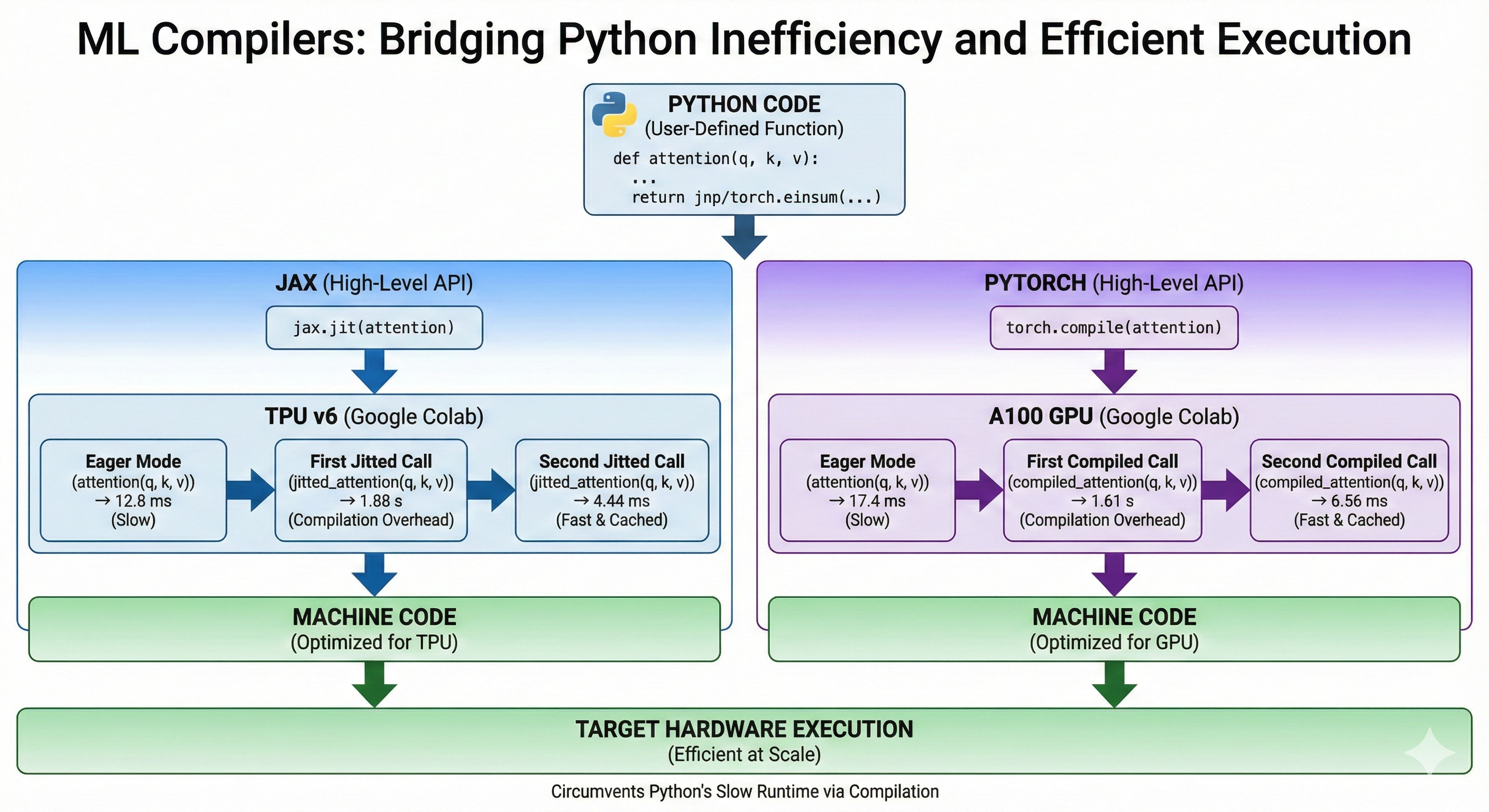
Python is a particularly inefficient programming language. Yet, it is used almost ubiquitously to develop massive models and deploy them efficiently at scale. How come?
ML frameworks circumvent Python's slow runtime by compiling the model's code into machine code for the target architecture just like the Rust compiler would. This allows us to write efficient code despite python.
High Level APIs
In this chapter, we will cover both Jax and PyTorch. They both provide an API to compile a Python function and make it more efficient. For now, we will only showcase the APIs. It the later subchapters, we will dive into the differences between Jax and PyTorch compilation processes and the different optimizations that the ML compilers perform.
Let's implement the attention mechanism in both Jax and PyTorch to demonstrate how the API works at a high level.
Jax
Jax offers the jax.jit method that takes a python function and a set of abstract inputs and compiles an optimized method for the function, inputs pair. Abstract inputs are composed of a dtype and a shape. The first call to the jitted function is slow because it needs to perform the compilation, the subsequent calls are very fast because the compilation is cached. Calling the same method with inputs of different dtype or shape will trigger a recompilation.
We are running this on a TPU v6 in Google Colab. We use block_until_ready otherwise, Jax would not wait for the computations to be complete on TPU before yielding back control to the CPU.
from jax import numpy as jnp
import jax

def attention(q, k, v):
  qk = jnp.einsum('btnh,bsnh->btns', q, k)
  scores = jax.nn.softmax(qk, axis=-1)
  return jnp.einsum('btns,bsnh->btnh', scores, v)

jitted_attention = jax.jit(attention)
Weights initialization
key_q, key_k, key_v = jax.random.split(jax.random.PRNGKey(0), 3)

shape = (32, 1024, 16, 256)

# Automatically on TPU in Jax
q = jax.random.normal(key_q, shape, dtype=jnp.bfloat16)
k = jax.random.normal(key_k, shape, dtype=jnp.bfloat16)
v = jax.random.normal(key_v, shape, dtype=jnp.bfloat16)
Runtime in Eager Mode
%%time
out = attention(q, k, v).block_until_ready()
stdout
Wall time: 12.8 ms
First jitted call
%%time
out = jitted_attention(q, k, v).block_until_ready()
stdout
Wall time: 1.88 s
Second jitted call
stdout
Wall time: 4.44 ms
PyTorch
PyTorch uses the torch.compile method. At a high level, it is very similar to jax.jit. Notice how similar the code is.
We are running this on an A100 in Google Colab.
import torch

def attention(q, k, v):
  qk = torch.einsum('btnh,bsnh->btns', q, k)
  scores = torch.nn.functional.softmax(qk, dim=-1)
  return torch.einsum('btns,bsnh->btnh', scores, v)

compiled_attention = torch.compile(attention)
Weights Initialization
# Explicitly set default device to GPU
device = torch.device("cuda")

shape = (32, 1024, 16, 256)

generator = torch.Generator(device=device).manual_seed(0)

q = torch.randn(shape, generator=generator, device=device, dtype=torch.bfloat16)
k = torch.randn(shape, generator=generator, device=device, dtype=torch.bfloat16)
v = torch.randn(shape, generator=generator, device=device, dtype=torch.bfloat16)
Runtime Eager Mode
%%time
out = attention(q, k, v)
# Equivalent of block_until_ready
torch.cuda.synchronize()
stdout
Wall time: 17.4 ms
First Compiled Call
%%time
out = compiled_attention(q, k, v)
# Equivalent of block_until_ready
torch.cuda.synchronize()
stdout
Wall time: 1.61 s
Second Compiled Call
stdout
Wall time: 6.56 ms
Why not just use another language?
There are efforts to create new languages for ML. For instance Julia which seems to have lost its momentum and Chris Lattner's Mojo which is too recent to tell.
The reasons Python is so commonly used in the ML community are mostly historical and cultural. The language has been around for more than 30 years, so it has a lot of mature and stable libraries that are commonly taught in universities. It is also easy to pick up and play with, making it ideal for quick iterations in research environments. At this point, Python's adoption is not about its inherent qualities but mostly about network effects, which are extremely difficult to compete against.
Jax vs PyTorch
While Jax's and PyTorch's APIs look similar, they handle compilation very differently. This matters a lot when writing code in either library and when thinking about performance.
Tracing (Jax)
Jax uses the tracing approach. When we we compile a Python method using jax.jit, we set a global variable called the Tracer. When our Python code encounters a Jax method, it appends an instruction to the global Tracer. At the end of our function, the Tracer has a full graph of instructions that it finally compiles.
This means that:
- The only code that will be compiled will be the
Jaxmethods we encountered during compilation. If..elsestatements andfor loopsare only evaluated at compile time and their evaluation will be constant at run time.- Runtime dependent control flow has to be implemeted using
JaxAPIs likejax.lax.condandjax.lax.fori_loop.
Another particularity is that jax.jit will compile your method for a specific set of input shapes and dtypes. Changing your input shape will force a recompilation of the program.
Furthermore, jitted methods are purely functional. We cannot mutate a value in-place. Performance Note: Although the API is functional (create new arrays), the compiler optimizes this into in-place updates under the hood, so you don't lose performance.
Let's illustrate what this means:
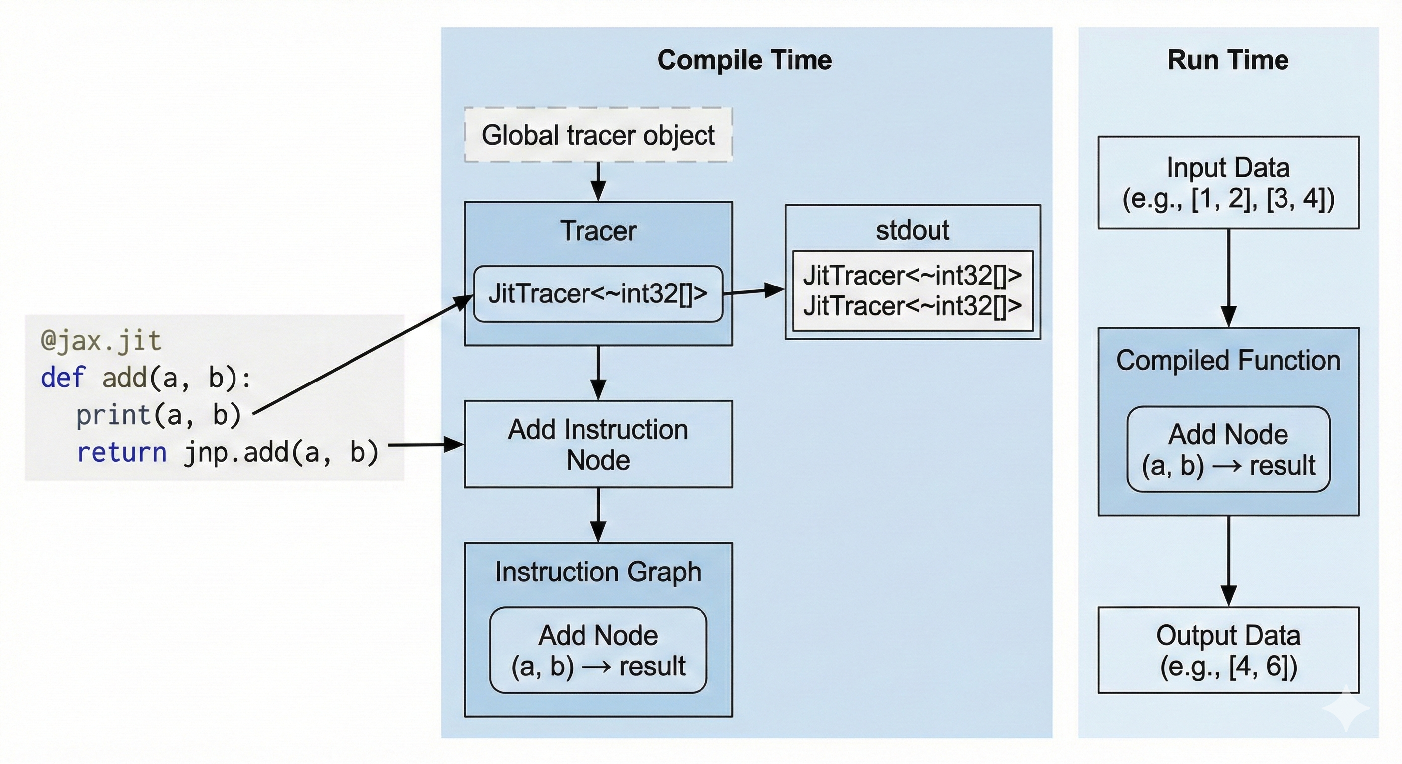
Printing (Jax)
import jax

@jax.jit
def add(a, b):
    print(a, b)
    return a + b

add(1, 2)
add(3, 4)
stdout
JitTracer<~int32[]> JitTracer<~int32[]>
The print statement is not a Jax method, so it only prints at compile time. We only have one stdout line even though we called the method twice because it only printed during compilation and the second call is cached. If we wanted to print actual runtime values, we would use jax.debug.print.
Runtime If Statement (Jax)
import jax

@jax.jit
def conditional(a, b):
    if a > b:
        return a
    return jnp.exp(b)

conditional(3, 4)
stderr
TracerBoolConversionError:
    Attempted boolean conversion of traced array with shape bool[].
We attempted to use a runtime value in an if statement, resulting in a compile-time error. We can fix this using jax.lax.cond to ensure that the Tracer knows about the if statement and compiles it.
import jax
import jax.numpy as jnp

@jax.jit
def conditional(a, b):
    return jax.lax.cond(a > b, lambda: a, lambda: jnp.exp(b))

# (Using floats because a and exp(b) must have the same type)
conditional(1., 2.)
Static Arguments
We can define static arguments to be passed to the method. These arguments will not be traced, however they can be used for control flow during compilation.
Let's look at this code:
from functools import partial
import jax
import jax.numpy as jnp

@partial(jax.jit, static_argnames=('add_residuals',))
def linear_layer(x, w0, add_residuals: bool = False):
    y = x @ w0
    # add_residuals is static so it can be used in the `if` statement
    if add_residuals:
        return x + y
    return y

x = jnp.ones((32, 128))
w0 = jnp.ones((128, 128))
When we compile the method with add_residuals = False, the Tracer never sees the x + y operation, so it never gets compiled and the Tracer never knows this line of code existed. If you call the function again with add_residuals = True, Jax MUST recompile the whole function.
We can even pass functions or complex objects as static arguments!
from typing import Callable

@partial(jax.jit, static_argnames=('activation',))
def linear_layer(x, w0, activation: Callable[[jax.Array], jax.Array] | None = None):
    y = x @ w0
    if activation:
        return activation(y)
    return y

x = jnp.ones((32, 128))
w0 = jnp.ones((128, 128))

linear_layer(x, w0, jax.nn.relu)
Bytecode Interception (PyTorch)
PyTorch's approach puts less weight on the developer. Any method that works in eager mode will also work with torch.compile. This is achieved by intercepting Python's bytecode and dynamically modifying it right before execution. This throws all of Jax's limitations out of the window.
Some Python operations cannot be compiled directly by torch.compile. For instance print or numpy calls. When torch.compile encounters these operations, it falls back to Python; we call this a Graph Break. Graph Breaks are slow and should be kept to a minimum to reach maximum performance.
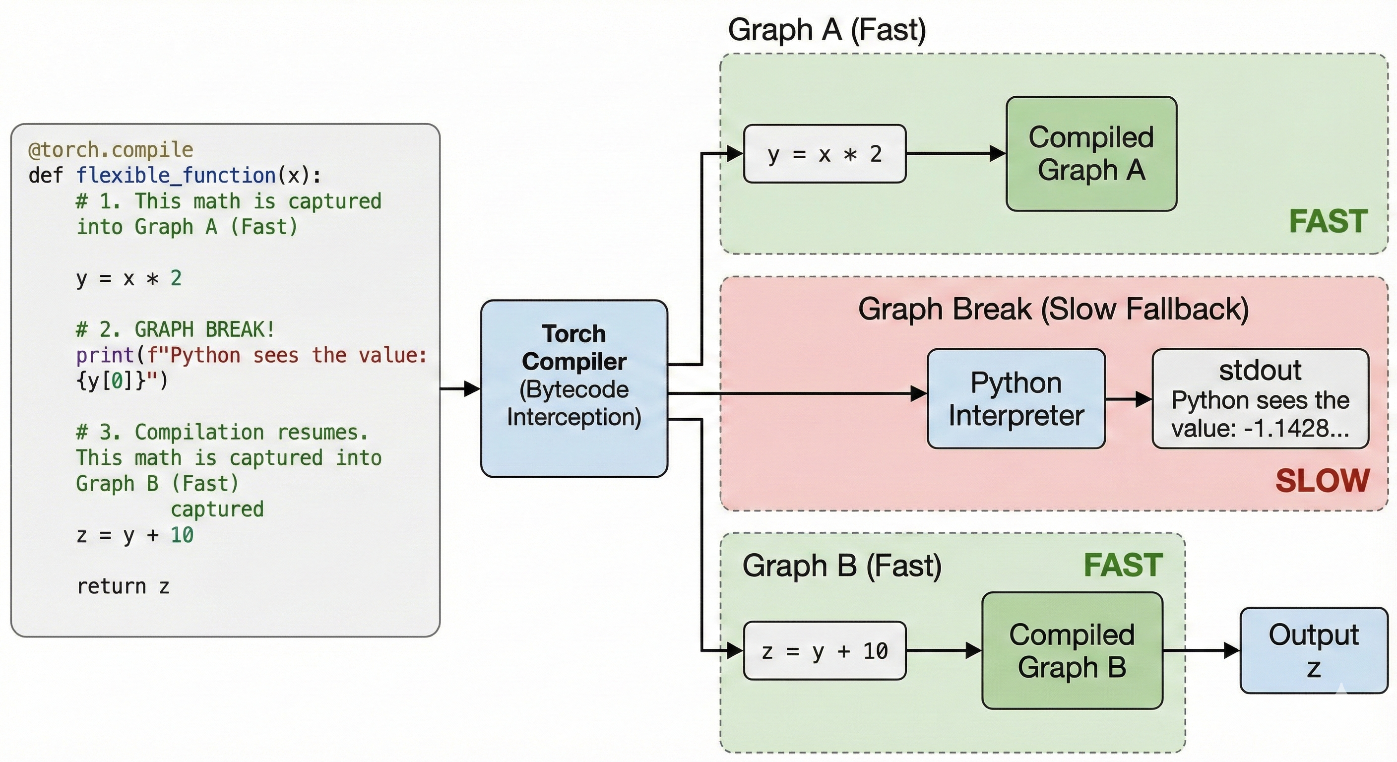
Printing (PyTorch)
import torch

@torch.compile
def flexible_function(x):
    # 1. This math is captured into Graph A (Fast)
    y = x * 2

    # 2. GRAPH BREAK!
    # The compiler pauses. Python executes this print.
    print(f"Python sees the value: {y[0]}")

    # 3. Compilation resumes. This math is captured into Graph B (Fast)
    z = y + 10
    return z

x = torch.randn(5)
flexible_function(x)
stdout
Python sees the value: -1.1428250074386597
We print the runtime value at the cost of a graph break.
Runtime If Statement (PyTorch)
import torch

@torch.compile
def conditional(a, b):
    if a.sum() > b.sum():
        return a
    return torch.exp(b)

a = torch.randn(5)
b = torch.randn(5)

conditional(a, b)
This code compiles without errors unlike Jax. However, it introduces a Graph Break. We can fix it by staying in graph with an API like torch.where.
Eager Mode
We need to first understand Eager Mode to understand how compilation improves perfomance on top of it.
Eager Mode is the standard execution model of Jax and PyTorch. When you run ML code without torch.compile or jax.jit, you are executing code on the CPU in the Python runtime, this code sends instructions to the GPU or TPU that actually performs the computations.
When you chain multiple operations one after the other, the CPU doesn't wait for the GPU/TPU to complete its task, it takes the next operation and already schedule it concurrently to the GPU/TPU's execution. When all operations have been scheduled, the CPU waits for the GPU/TPU's work to be over.
Let's have a look at this PyTorch function running on GPU.
import torch
from torch.profiler import profile, record_function, ProfilerActivity

def complex_activation(x, y):
    # Eager PyTorch launches 6 separate kernels for this:
    # Read/Write memory 6 times!
    a = torch.sin(x)
    b = torch.cos(y)
    c = a * b
    d = c + x
    e = d * y
    return torch.relu(e)
The Bottleneck: In Eager Mode, every line of code above requires reading data from the GPU's memory (HBM), computing, and writing the result back. We are constantly moving data back and forth, which is often slower than the math itself.
We profile it using the torch profiler
N = 20 * 1024 * 1024
x = torch.randn(N, device='cuda')
y = torch.randn(N, device='cuda')

torch.cuda.synchronize()
# Warmup
complex_activation(x, y)
torch.cuda.synchronize()

with profile(
    activities=[ProfilerActivity.CPU, ProfilerActivity.CUDA],
    record_shapes=True,
    with_stack=True
) as prof:
    with record_function(f"run"):
      complex_activation(x, y)
    torch.cuda.synchronize()
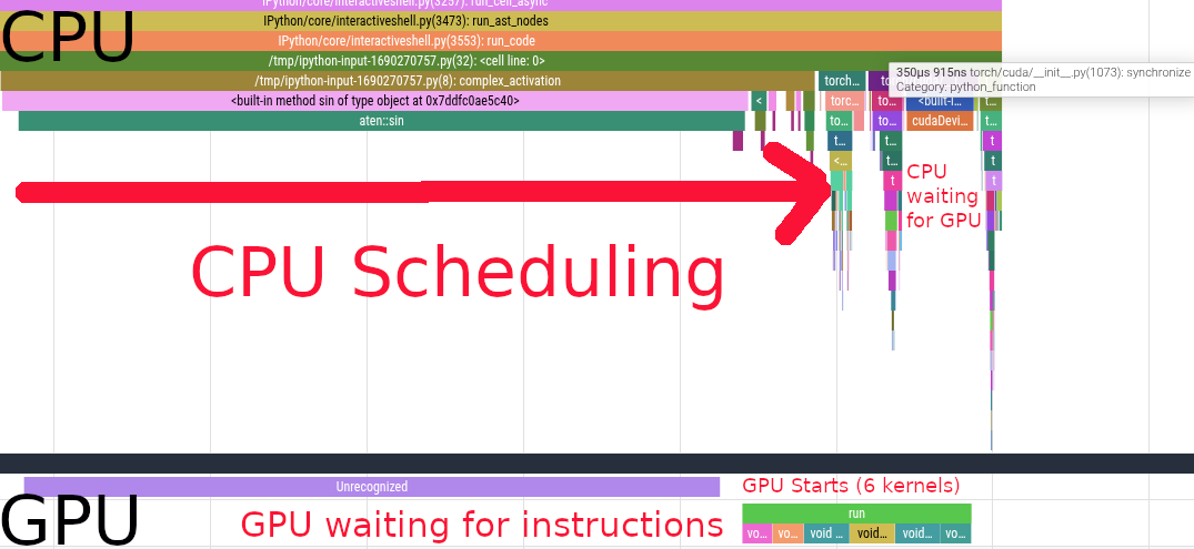
We see the CPU scheduling the first sin call. Scheduling the first kernel is very slow because of the synchronization overhead. After that, we see a bunch of other kernels being scheduled on the CPU side, those are cos, a * b, c + x, d * y and relu.
We see that the GPU starts working while the CPU is still scheduling instructions. After scheduling, the CPU starts waiting for the GPU to complete its work. The GPU executes 6 different kernels in \(731\mu s\).
Optimizations
When running code in Eager Mode, PyTorch and Jax see function calls one at a time. They cannot reason holistically about how these functions interact together. So while each individual function is written optimally, the transitions between functions are suboptimal.
On the contrary, jax.jit and torch.compile allow their compilers to see the whole code ahead of time. This gives them the opportunity to fuse, rewrite, and eliminate code optimally.
Kernel Fusions
Let's take another look at the code from the previous chapter.
def complex_activation(x, y):
    # Eager PyTorch launches 6 separate kernels for this:
    # Read/Write memory 6 times!
    a = torch.sin(x)
    b = torch.cos(y)
    c = a * b
    d = c + x
    e = d * y
    return torch.relu(e)

opt_activation = torch.compile(complex_activation)
In Eager Mode, we scheduled 6 different kernels one after the other. This means that the GPU had to load from HBM the whole array each time and then write it back in between kernels.
When we compile the code, PyTorch fuses all the kernels, allowing the GPU to load the arrays x and y from HBM once, and applying all the computations once from fast memory.
Here's the flame graph
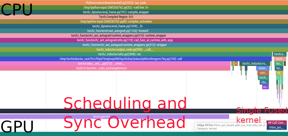
We now have a single kernel instead of 6. Bringing the latency down from \(731\mu s\) to \(144\mu s\).
Buffer Reuse
When an array is read once and not needed after, ML compilers can reuse the memory space instead of constantly reallocating. This saves both memory and latency by increasing cache locality.
In the previous example, compilers need to allocate for x and y. Then
- We have to allocate
aandbbecausexandyare needed later a(orb) can be overwritten withcbecause they are not reusedxcan be overwritten withdycan be overwrittenewhich can be muttated in place before returning
Relayout
ML compilers are able to reason about the best layout for your operations. For instance, the MXU on the TPU operates on array of shape \((8, 128)\) at least. If you have an einsum with an input shape \((64, 4, 1024)\), the 4 being a non contracted batch dimension like the number of heads in attention, jax.jit will transpose your array to \((4, 64, 1024)\) under the hood, making full use of the MXU.
Dead Code Elimination
Sometimes, we write code that is not needed for anything. It is not returned, nor does it have any effects (like print). This code is completely safe to be removed from the program.
For instance, in this example the x @ gating1 call is absent from the flame graph
def mlp(x, gating0, gating1, linear):
    y = x @ gating0
    # x @ gating1 is never accessed, this computation is useless
    # it is eliminated by the compiler
    unused = x @ gating1

    y = torch.nn.functional.relu(y)
    out = y @ linear
    return out

compiled_mlp = torch.compile(mlp)

device = torch.device("cuda")


generator = torch.Generator(device=device).manual_seed(0)

b = 512
d = 2048
f = 2 * d

x = torch.randn((b, d), generator=generator, device=device, dtype=torch.bfloat16)
gating0 = torch.randn((d, f), generator=generator, device=device, dtype=torch.bfloat16)
gating1 = torch.randn((d, f), generator=generator, device=device, dtype=torch.bfloat16)
linear = torch.randn((f, d), generator=generator, device=device, dtype=torch.bfloat16)

There are only 2 gemm kernel calls
Backward Pass
ML frameworks implement auto differentiation for us, so we usually do not need to implement the backward pass ourselves. Nonetheless, it is important to understand how the gradients are propagated to be able to reason about memory usage and the computational overhead of the backprop.
What are the Forward and the Backward Pass?
The Forward pass is the "main formula" of the model. It is the primary computation of the model, transforming inputs to outputs. It is executed during both inference (to get predictions) and training (to compute the loss).
The Backward Pass (Backpropagation) is the chain rule of calculus applied in reverse. It computes the gradient of the loss function with respect to every parameter in the model. These gradients indicate the direction and magnitude to adjust each parameter to minimize error.
The forward pass produces predictions. During training, these predictions are compared to a ground truth value to calculate a loss. The backward pass produces gradients, or directions for each parameter in the model. The gradients are consumed by the optimizer to update the weights used in both the forward and the backward pass.
How is it computed?
Most functions in ML are differentiable (or have defined subgradients for points like x=0 in ReLU). Therefore, when ML frameworks developers implement a function, they implement its forward and backward methods.
A basic example using jax.grad, the derivative of the Sine function sin is simply the Cosine cos. When we apply jax.grad to jnp.sin, jax will internally call jnp.sin.backward (not the exact internal name), which is jnp.cos.
import jax.numpy as jnp

grad_sin = jax.grad(jnp.sin)
grad_sin(0.2) == jnp.cos(0.2)
Let's take a look at a more complex example:
import jax
import jax.numpy as jnp

key0, key1, key2 = jax.random.split(jax.random.key(0), 3)

b, d, f = 16, 64, 32
x = jax.random.normal(key0, (b, d))
w_0 = jax.random.normal(key1, (d, f))
w_1 = jax.random.normal(key2, (f, d))

def mlp(args):
  x, w_0, w_1 = args
  z = x @ w_0
  z_relu = jax.nn.relu(z)
  out = z_relu @ w_1
  return 0.5 * jnp.sum(out ** 2)

grad_mlp = jax.grad(mlp)

# jax.grad only returns the gradients of the first argument
# so we pass all our arguments as a tuple
grad_mlp((x, w_0, w_1))
This is a classic 2 layers MLP with a ReLU activation in between. \[\text{ReLU}(x W_0) W_1\]
- The
Forward Passsimply executes the code we wrote. - The
Backward Passtakes the output of theForward Passand executes the backward methods in reverse order by propagating gradients backward. - Some derivatives require the original activation from theForward passso we need to individually store them during theforward call.
Walking through the backward pass
0.5 * jnp.sum(out ** 2)The derivative is simplyoutout = z_relu @ w_1Here we need to compute the gradients ofw_1which will be used to updatew_1by the optimizer and the gradients ofz_reluthat will be backpropagated.dL/dW1 = z_relu.T @ grads((b, f).T @ (b, d) -> (f, d))dL/dZ_relu = grads @ w1.T((b, d) @ (f, d).T -> (b, d))
z_relu = jax.nn.relu(z)ReLUis defined asrelu(x) = max(0, x). Its derivative is therefored_relu(x) = 0 if x <= 0 else 1. We then multiply the derivative with the gradients.- Performance Note: Storing values in
HBM(High Bandwidth Memory) is expensive. For element-wise operations like ReLU, it is often faster torecomputethe activation during the backward pass using the cached input (z) rather than storing the output (z_relu) and reading it back. This is known asactivation recomputationorrematerialization.
- Performance Note: Storing values in
z = x @ w_0. Just like for layer 1:dL/dW0 = x.T @ grads((b, d).T @ (b, f) -> (d, f))dL/dx = grads @ w0.T((b, f) @ (d, f).T -> (b, d))
First let's rewrite the MLP implementation to cache the intermediate activations:
def mlp_activations(x, w_0, w_1):
  activations = [x]
  z = x @ w_0
  activations.append(z)
  z_relu = jax.nn.relu(z)
  activations.append(z_relu)
  out = z_relu @ w_1
  activations.append(out)
  return 0.5 * jnp.sum(out ** 2), activations
Now let's implement the backward pass:
def manual_mlp_grad(x, w_0, w_1):
  # Forward
  _, activations = mlp_activations(x, w_0, w_1)

  # Pop out, shape (b, d)
  out = activations.pop()

  # 1. Derivative dL/dOut = out
  grads = out

  # 2. Derivative of Layer 1
  z_relu = activations.pop()
  # dL/dW1
  grads_w_1 = z_relu.T @ grads
  # dL/dZ_relu
  grads_z_relu = grads @ w_1.T

  # 3. Derivative of ReLU
  z = activations.pop()
  grads_z = jnp.where(z > 0, 1, 0) * grads_z_relu

  # 4. Derivative of Layer 0
  x = activations.pop()
  # dL/dW0
  grads_w_0 = x.T @ grads_z
  # dL/dx
  grads_x = grads_z @ w_0.T

  return grads_x, grads_w_0, grads_w_1
Correctness check:
import numpy as np

manual_out = manual_mlp_grad(x, w_0, w_1)
jax_out = grad_mlp((x, w_0, w_1))

for manual, autograd in zip(manual_out, jax_out):
  np.testing.assert_allclose(manual, autograd)
Performance Implications
Flops
As we have seen, each matrix multiplication in the forward pass requires two matrix multiplications in the backward pass. Hence, the number of flops in the backward pass can easily be approximated as twice the flops of the forward pass.
Memory Usage
Since we need to store the intermediate activations during the forward pass, our model requires a lot more memory during training than during inference. A common rule of thumb is that Training memory is ~3x-4x Inference memory for the same batch size, primarily due to the need to store these intermediate activations. Furthermore, constantly writing and reading previous activations saturates the memory bandwidth which slows down prefetching of other parameters.
It is crucial to study which activations are being cached, and actively find opportunities for recomputations when appropriate. Either to free up memory or to speed up the step time.
On-Chip Parallelism
Machine Learning workloads require more and more computational power as we scale the number of parameters, the context lengths, and the amount of data we ingest. At the same time, chip design has hit a plateau; it is getting prohibitively expensive to increase the number of operations a chip can do per second. Furthermore, memory latency and bandwidth have not been keeping up with the increases in compute speed, implying that computational power cannot be fully leveraged because the data cannot be moved as fast as it is being processed. We cannot rely on faster chips, so we instead rely on the chips doing more at the same time either by doing multiple operations at once or having multiple cores working together in parallel.
Sequential execution model
Traditional chips were thought of as having two main blocks; the memory (RAM) and the Central Processing Unit (CPU.)
Traditional software is usually written with this implied model:
- Load some scalars from RAM to the CPU
- Do some operations on the CPU
- Write back the output of those operations to RAM
- Repeat for the next instruction
While this model is great and allowed us to write most of the software running the world today; it has long become incoherent with the way chips actually process data. We let the compilers and the chips themselves rewrite our code to make better use of the actual capabilities of the hardware; mostly through different levels of parallelism and better memory access patterns.
The different levels of on-chip parallelism
Modern chips are all inherently parallel. Whether they are GPUs, TPUs, or modern CPUs. They also all feature different types of parallelism that need to be exploited to maximize the chip's utilisation. Exploiting these mechanisms is not always explicit because compilers are reasonably good at leveraging target architectures's features. Some chips are also capable of rewriting the machine code they receive before executing it.
IO parallelism
The processing unit and the memory are two independent units. Therefore, the processor is able to perform computations independently of the memory reads and writes. For instance, it can request some data from RAM as well as perform an addition between two numbers it has already loaded while waiting for the data to be received. This means we can potentially completely overlap computation times with memory movements. In our execution model, steps 1, 2, and 3 can all be executed in parallel.
Single Instruction Multiple Data (SIMD)
Most modern chips are capable of executing a single instruction on multiple elements at once. This can mean adding two vectors with one another in one cycle, reducing (ie. summing) a vector into a scalar, or even running a matrix dot product within specialized Arithmetic Logic Units (ALUs) in TPUs' and GPUs' tensor cores.
- Modern x86 chips feature AVX registers
- TPUs have MXUs for matrix dot products, VPUs for elementwise vectorized operations, and XLUs for reductions
- GPUs have tensor cores for matrix dot products
Coming back to our execution model. Instead of executing one operation at a time on scalars, we instead perform as many operations as we can in parallel within a SIMD unit and also load more data at once since our registers are larger.
Instruction Level Parallelism
As we have mentioned, modern chips possess multiple circuits that specialize in the handling of different data types and operations. For instance, TPUs have MXUs and VPUs. Some of these circuits can also be used independently. For instance, we could compute a dot product on the MXU, and apply a ReLU activation at the same time on the VPU (more specifically, perform a dot product, write the output to the VPU, do the next dot product at the same time as we apply ReLU on the VPU.)
Multiple threads of execution
Finally, modern architectures usually feature multiple processing units that can execute operations independently of one another. This is the main differentiator of GPUs which possess thousands of cores that can all execute operations in parallel on different data addresses. This model comes with additional complexities such as the need to synchronize data across cores safely and efficiently.
Coming back to the original model, we now execute the model multiple times in parallel.
Comparison of On-Chip Parallelism
| Parallelism Type | Core Concept | ⚙️ Hardware Example | 💻 Software Abstraction | 👤 Who Implements This? |
|---|---|---|---|---|
| IO parallelism | Hiding memory latency by performing computation while waiting for data to be fetched. | GPU warp schedulers swapping threads stalled on memory reads; hardware prefetchers. | Optimized kernels (e.g., in cuDNN, XLA). | Chip Hardware (schedulers) & Compiler (instruction scheduling). |
| SIMD (Single Instruction, Multiple Data) | One instruction operating on many data elements (a vector) at once. | GPU Tensor Cores (for matrices), TPU MXUs, CPU AVX registers. | Vectorized code (e.g., a + b on tensors), torch.matmul. | Compiler / Library (e.g., cuDNN, XLA). The programmer enables this by using high-level vector/matrix ops. |
| Instruction-Level Parallelism (Using Multiple ALUs) | Using different, specialized execution units (ALUs) within a core at the same time. | A TPU pipelining work from its MXU (matrix) to its VPU (vector). | Kernel Fusion (e.g., matmul + relu in one operation). | Compiler (e.g., jax.jit, XLA). The chip hardware makes it possible. |
| Multithreading / Multicore (MIMD / SIMT) | Multiple processing units (cores) executing instructions independently. | Multi-core CPU (MIMD), thousands of CUDA Cores on a GPU (SIMT). | Data Parallelism (splitting a batch over cores) or Model Parallelism. | Programmer & Library (e.g., CUDA, which manages threads for kernels). |
Estimating Performance
We want to answer the following question: "Given my code and my chip, what is the fastest theoretical time this function should take?"
We can simply model it, by assuming we can overlap all the components involved in the operation (Memory, Tensor Cores, etc), the theoretical fastest time is going to be the time of the slowest component.
How to Estimate our Performance?
We need to figure out which part of the chip will be taking the largest amount of time.
Therefore, we need:
- How much time will it take the ALUs to execute all computations?
- How long will we spend loading the data from the main memory to the ALUs?
- What is the maximum of these two values?
Let's start with 1. Typically, we will estimate a simple dot product. The flops of a dot product are computed as such:
for an mk,kn->mn dot product

flops = m * k * n * 2
Now we need to divide the number of flops by the theoretical limit of the machine to get the peak theoretical compute performance.
compute_seconds = flops / flops_per_second(chip)
Now, let's compute the time it will take to load the memory onto the ALUs and to write the output back.
let's call the left hand side "lhs" and the right hand side "rhs".

total_memory_bytes = (m * k * bytes_per_element_lhs) + (k * n * bytes_per_element_rhs) + (m * n * bytes_out)
The time it should take to load the memory will be
memory_time_seconds = total_memory_bytes / memory_bandwidth_seconds(chip)
Our theoretical run time will be:
max(compute_seconds, memory_time_seconds)
Practical Example
Let's estimate the run time of a dense MLP subblock of a transformer on an A100 Nvidia GPU.
The specs for the GPU are as followed:
| Specification | A100 40GB PCIe |
|---|---|
| FP32 | 19.5 TFLOPS |
| BFLOAT16 Tensor Core | 312 TFLOPS |
| GPU Memory Bandwidth | 1,555 GB/s |
@torch.compile
def mlp(x, w1, w2, wlinear):
  x1 = x @ w1
  x1 = torch.nn.ReLU()(x1)
  x2 = x @ w2
  x = x1 * x2
  out = x @ wlinear
  return out
Let's say that our d_model is 4096 and our hidden dimension is 8192. Let's start with a batch size of 32.
- Tensore Core We have 2 dot products
bd,df->bfand onebf,fd->bd,flops = 32 * 4096 * 8192 * 2each. We calculate the matmul time against the 312 TFLOPS BF16 Tensor Core spec, as these are specialized for matrix operations.
tc_time_secs = flops * 3 / tensor_core_flops_per_sec
tc_time_secs = 32 * 4096 * 8192 * 2 * 3 / (312 * 1e12)
tc_time_secs = 0.00002065
- CUDA Cores We have the ReLU and the elementwise multiplication
x1 * x2bot of these operations takeb * fflops. We calculate the ReLU and element-wise ops against the 19.5 TFLOPS FP32 CUDA Core spec, as Tensor Cores cannot run these.
cuda_time_secs = 32 * 8192 * 2 / (19.5 * 1e12)
cuda_time_secs = 2.69e-8
- Memory load times We have to load
x,w1,w2, andwlinear. We have to write the output. We assume we do not have to write and read the intermediate activations... This is a key benefit of usingtorch.compile, which performs kernel fusion. It merges thematmul,ReLU, andelement-wise multiplyoperations into a single kernel, so the intermediate results (likex1andx2) never have to be written to or read from the main (HBM) memory.
bf16_bitsize = 2

x_size = 32 * 4096 * bf16_bitsize
out_size = x_size
w_size = 4096 * 8192 * bf16_bitsize
total_size = x_size + 3 * w_size + out_size

memory_time_secs = total_size / (1.555 * 1e12)
memory_time_secs = 0.000129
- Estimation
estimation = max(tc_time_secs, cuda_time_secs, memory_time_secs)
estimation = 0.000129
Our estimation is ~129µs. Let's run it into colab on an A100.
mlp(x, w_gating_1, w_gating_2, w_linear)
%timeit mlp(x, w_gating_1, w_gating_2, w_linear)
191 µs ± 8.17 ns per loop (mean ± std. dev. of 7 runs, 10000 loops each)
The actual runtime is 48% slower than our estimate, which is expected because of inefficiencies like kernel launch overheads, synchronization, and any small gaps between the fused operations.
Roofline Model
The roofline model measures the peak throughput of the chip.
The Core Concept: Arithmetic Intensity
Arithmetic Intensity (AI): is a characteristic of your algorithm. It's the ratio of compute to memory access.
AI = flops / data_moved
The achievable performance will be expressed as
perf = min(peak_flops, peak_bandwidth * AI)
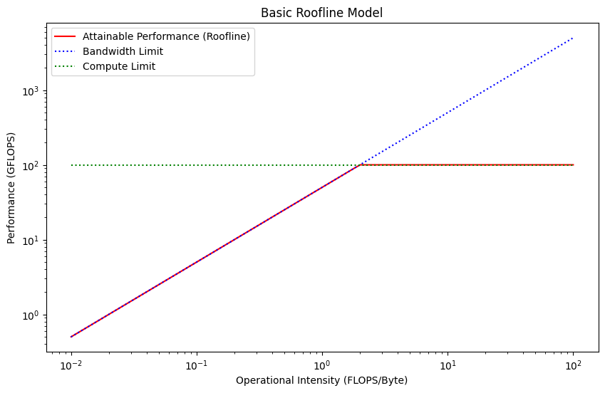
Takeaway
The key takeaway is that as long as we are memory bound, increasing the arithmetic intensity will yield significant throughput improvements. When we are compute bound, increasing the arithmetic intensity, will commensurably increase the latency, resulting in no throughput gains. Therefore, we always want to be compute bound for throughput, but any point on the "flat part" of the roofline will be as efficient as any other.
Practice Questions
Does my runtime make sense?
You will be shown some code. You will be asked whether the runtime of the code makes sense given the performance characteristics of a chip. Compute the expected runtime and compare it to the measured runtime.
If the observed runtime is an order of magnitude slower than expected, look for inefficiencies.
- Are the kernels compiled and fused?
- Is the data properly allocated on the GPU or is it copied to and from the CPU?
- Are we using some non vectorized operations that are not being properly fused?
- Are we materializing some intermediate computations that don't have to be?
If the observed runtime is close expected, you will have to propose ideas to make the runtime faster.
- If we are memory bound, we should try lowering the memory loads by downcasting from
fp32tobf16, or frombf16toi8/i4through quantization. - If we are compute-bound, we have successfully saturated the chip's compute units and achieved peak throughput. At this point, you can't get more throughput. The conversation now shifts to latency. To lower latency, you must reduce the total work, which means either:
- Reducing the batch size, which will trade some of our hard-won throughput for lower latency.
- Reducing the FLOPS of the model itself through techniques like pruning or distillation.
Performance Modelling
You will be shown a model's architecture, and given a chip's specification.
- You will be asked to model the runtime of the model given different batch sizes.
- Compute the expected runtime as we've seen before.
- You will have to compute the amount of memory required for each batch size.
- You will be tasked with finding the optimum batch size to maximize throughput.
- According to the roofline model, this corresponds to the smallest batch size that makes the operation compute-bound. This is the "knee" or "ridge point" of the roofline. Any batch size larger than this will only increase latency without any corresponding gain in throughput, as you're already at
Peak_FLOPS. - Find which batch size is compute bound by simply figuring out which batch size has a higher compute time than memory time.
- The optimum batch size should not use more memory than available on the chip.
- According to the roofline model, this corresponds to the smallest batch size that makes the operation compute-bound. This is the "knee" or "ridge point" of the roofline. Any batch size larger than this will only increase latency without any corresponding gain in throughput, as you're already at
Distributed Computations
When a single chip is not enough, we can use multiple chips working together to either lower our latency, to increase the size of our model, or to increase our batch size.
As we scale our model to large number of parameters, we end up using more memory than we can fit on a single device. At this point, we need to add another device to make our model's weights fit.
There are also scenarios where parameters do fit on a single device, but we want to process massive amounts of data. This also forces us to distribute our computations.
Collective Operations and Sharding
We will end up distributing our computations differently depending on the model's architecture, the workload, the type, and the number of devices we have access to.
We typically call "sharding" the act distributing an axis of a model on multiple devices.
There are three Collective Operations typically used to synchronize the state of computations across devices, or to move from one sharding to another; All-Gather, All-Reduce, and All-To-All. We will introduce them, then explore how they are used in different scenarios.
Distributed Operations
Let's first review the three most important distributed operations.
All-Gather
An All-Gather operation takes an array with an axis distributed over multiple chips, and exchanges the data from each chip to each other chip such that each chip ends up with a full view of the data. It basically "unshards" one or several axes.
For instance, a vector of length 256 whose single axis would be sharded over 4 devices:
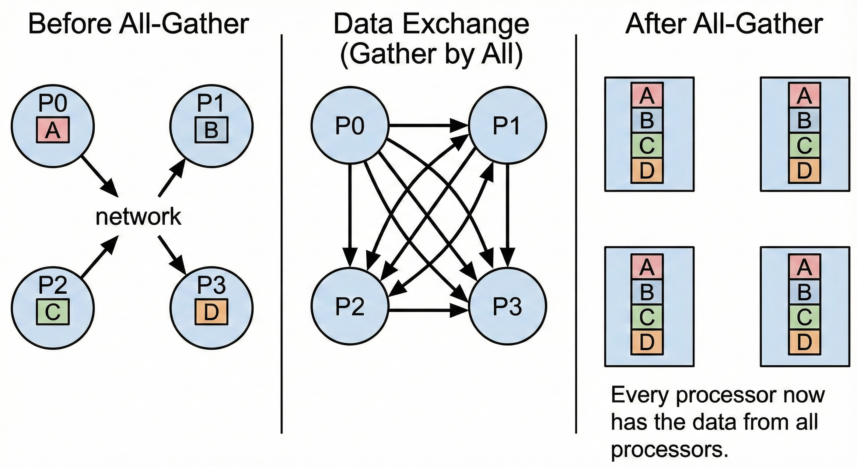
Each chip initially holds 64 different elements. After the All-Gather, they all have a replicated view of the same 256 elements.
All-Reduce And Reduce-Scatter
An All-Reduce operation takes a tensor from every device, combines them using an operator (typically sum), and returns the full result to every device.
For instance, a vector of length 256 whose single axis would be sharded over 4 devices:
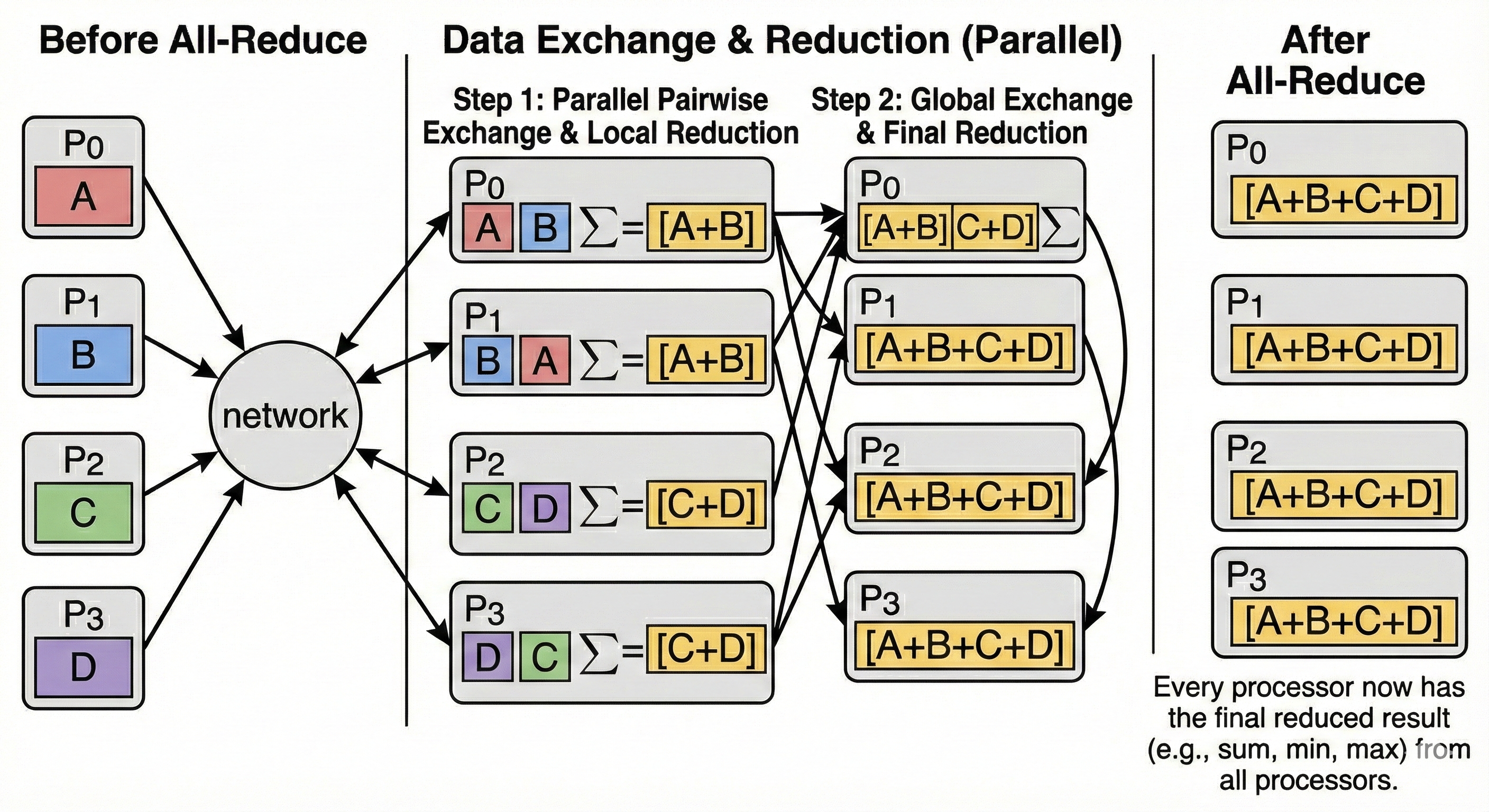
Each TPU initially holds 64 unique elements, after the All-Reduce, they all hold a vector which is replica of the sum of the vectors initially held by each chip.
Reduce-Scatter
A Reduce-Scatter is a "fused" operation. It performs the same reduction (sum) as All-Reduce, but instead of returning the full result to everyone, it scatters (shards) the result across the devices.
Conceptually, Reduce-Scatter is equivalent to an All-Reduce followed immediately by a Scatter (slice), but it is much more bandwidth-efficient because the full sum is never fully materialized on any single device.
All-To-All
All-To-All is a more general operation where each device exchanges data with all other devices. It is typically used when indexing a sharded array. Custom All-To-All can exchange different elements with all other devices depending on some runtime condition, this is the case for Mixture of Experts.
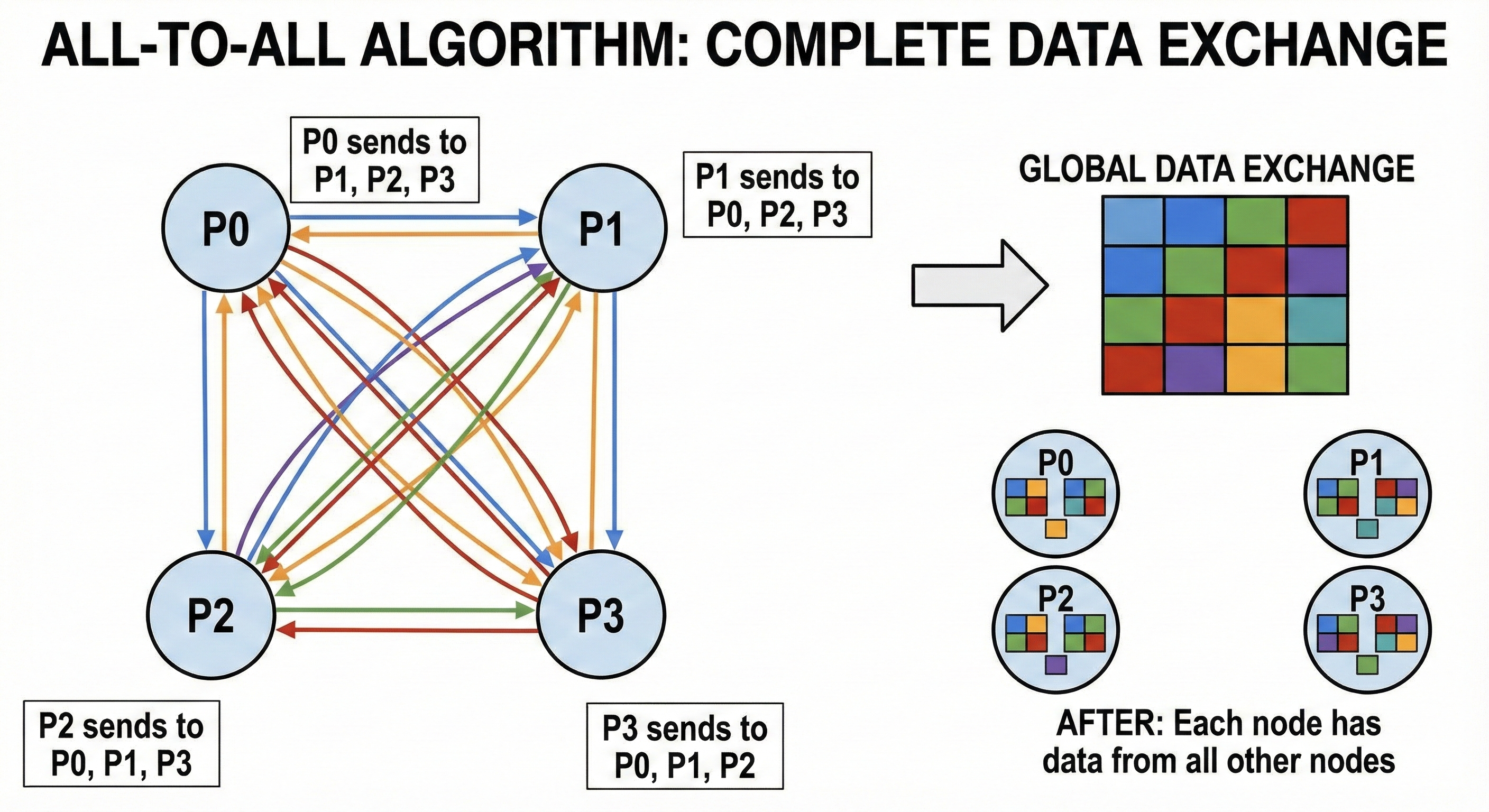
Sharding Strategies (intro)
We can split computations and data across devices to reduce the flops and the amount of memory needed per device. There are many ways we can split data and computations across devices. This chapter explores common sharding strategies.
Pseudo API
We will illustrate this chapter using a fake distributed API over numpy. This API contains all the building blocks required to enable distributed computations. The code snippets would conceptually be run on all devices in parallel. Devices are assigned a device_id to differentiate.
The API revolves around an abstract class that we have to inherit from. We have to implement 3 methods ourselves load_checkpoint, forward and backward.
The API provides pre implemented methods device_id, num_devices, barrier, send, receive, all_gather, all_reduce, all_to_all.
We also have an inference_loop method that simply loops over a stream of inputs and streams back the outputs to an output stream.
We do not provide the loss function and simply assume it is separately provided by the optimizer API.
from abc import ABC, abstractmethod
import numpy as np
import numpy.typing as npt
from io import Reader, Writer

class ShardedEngine(ABC):

    @property
    def device_id(self) -> int:
        """The rank of the current device."""
        ...

    @property
    def num_devices(self) -> int:
        """Total number of devices in the cluster (World Size).""" npt.ArrayLike
        ...

    def barrier(self) -> None:
        """Blocks until all devices reach this line."""
        pass

    # --- Point-to-Point Communication ---
    def send(self, dest_id: int, arr: npt.ArrayLike) -> None:
        ...

    def receive(self, src_id: int) -> npt.ArrayLike:
        ...

    def send_async(self, src: npt.ArrayLike, dst: npt.ArrayLike, target_device_id: int) -> Future:
        ...

    # --- Collective Communication ---
    def all_gather(self, arr: npt.ArrayLike, axis: int = 0) -> npt.ArrayLike:
        """Concatenates arrays from all devices along the specified axis."""
        ...

    def all_reduce(self, arr: npt.ArrayLike, op: str = 'sum') -> npt.ArrayLike:
        """Reduces arrays from all devices (e.g., sum) and broadcasts the result."""
        ...

    def all_to_all(self, arr: npt.ArrayLike, axis: int = 0) -> npt.ArrayLike:
        """Scatters chunks of the array to different devices."""
        ...

    # --- Model Lifecycle ---
    @abstractmethod
    def load_checkpoint(self, params: dict[str, npt.ArrayLike]) -> None:
        ...

    @abstractmethod
    def forward(self, x: npt.ArrayLike) -> npt.ArrayLike:
        ...

    @abstractmethod
    def backward(self, grads: npt.ArrayLike) -> dict[str, npt.ArrayLike]:
        ...

    def inference_loop(self, input_stream: Reader[npt.ArrayLike], output_stream: Writer[npt.ArrayLike]) -> None:
        for x in iter(input_stream):
            output_stream.write(self.forward(x))
Unsharded Example
Let's start with an unsharded example on a single device. We will start with a 2 layers model with a ReLU activation in between. \[\text{ReLU}(x W_0) W_1\]
def relu(x):
    return x * (x > 0)

class SingleDevice(ShardedEngine):

    def __init__(self, model_dim: int, hidden_dim: int):
        self.w0 = np.zeros((model_dim, hidden_dim), dtype=np.float32)
        self.w1 = np.zeros((hidden_dim, model_dim), dtype=np.float32)
        # Context tape to store activations for backward pass
        self.activations = []


    def load_checkpoint(self, params: dict[str, npt.ArrayLike]) -> None:
        # Load weights into local memory
        self.w0[...] = params['layer_0/weights'][...]
        self.w1[...] = params['layer_1/weights'][...]

    def forward(self, x: npt.ArrayLike) -> npt.ArrayLike:
        # 1. Save Input
        self.activations.append(x)

        # 2. Linear Layer 0
        # (Batch, Model) @ (Model, Hidden) -> (Batch, Hidden)
        z = np.einsum('bd,df->bf', x, self.w0)

        # 3. Activation
        self.activations.append(z) # Save pre-activation for the backward pass
        x = relu(z)

        # 4. Linear Layer 1
        # (Batch, Hidden) @ (Hidden, Model) -> (Batch, Model)
        out = np.einsum('bf,fd->bd', x, self.w1)
        return out

    def backward(self, grads: npt.ArrayLike) -> dict[str, npt.ArrayLike]:
        """
        grads: Incoming gradient dL/d(Output) of shape (Batch, Model_Dim)
        """
        # --- Backprop Layer 1 ---
        # Retrieve input to Layer 1 (Output of ReLU)
        # Shape: (Batch, Hidden)
        z = self.activations.pop()
        h_relu = relu(z)

        # dL/dW1 = h_relu.T @ grads
        w1_grad = np.einsum('bf,bd->fd', h_relu, grads)

        # Propagate gradient to h_relu: dL/dh = grads @ W1.T
        grads = np.einsum('bd,fd->bf', grads, self.w1)

        # --- Backprop ReLU ---
        # Apply derivative of ReLU: 1 if h > 0 else 0
        grads = grads * (z > 0)

        # --- Backprop Layer 0 ---
        # Retrieve input to Layer 0 (Original X)
        # Shape: (Batch, Model)
        x_input = self.activations.pop()

        # dL/dW0 = x_input.T @ grads
        w0_grad = np.einsum('bd,bf->df', x_input, grads)

        return {'layer_0/weights': w0_grad, 'layer_1/weights': w1_grad}
Data Parallelism
Data Parallelism (specifically Distributed Data Parallel or DDP) is the most common scaling strategy. It is simple: We shard the data by splitting it over multiple chips, but we replicate the model.
Let's explore this einsum:
out = torch.einsum('bd,df->bf', activations, weights)
Let's set b to 5120, d to 2048 and f to 1024. If we have 2 GPUs, each GPU will see one half of b (2560 vectors of size d each) and have a full replica of the weights.
In a forward pass, this means we never have to synchronize and we just run half our batch on a chip, and another half on the other chip. During the backward pass, we have to average the gradients from each GPU (using an all-reduce) to update our weights with the same value and maintain them replicated.
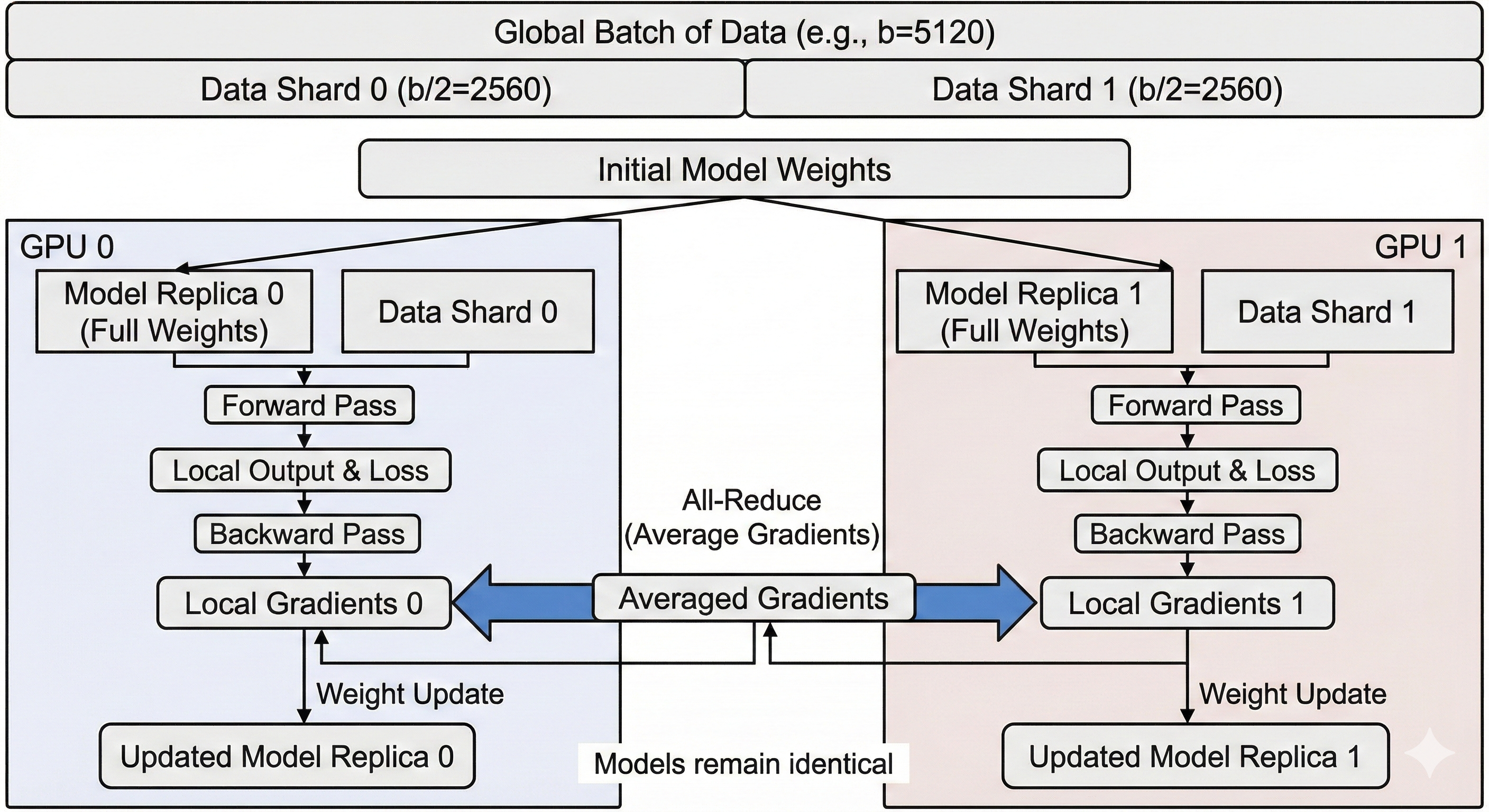
The Limit: Memory Redundancy
The main limitation of standard Data Parallelism is Memory. Because every GPU must hold a full copy of the weights, the gradients, and the optimizer states, the maximum model size is limited to what fits on a single GPU.
If your model is 80GB and your GPU has 40GB of VRAM, you cannot use standard Data Parallelism, even if you have 100 GPUs.
| Feature | Impact | Why? |
|---|---|---|
| Implementation | ✅ Easy | Supported natively (e.g., PyTorch DDP). It requires almost no code changes; you just wrap the model and the framework handles the gradient synchronization. |
| Throughput | ✅ High | Ideally provides linear scaling. If you double the chips, you process double the data per second (until network limits are reached). |
| Memory | ❌ Low | The major bottleneck. Every chip must store a full replica of the parameters, optimizer states, and gradients. You cannot train a model larger than what fits on a single chip. |
| Communication | ⚠️ Medium | Requires an All-Reduce of gradients after every backward pass. While bandwidth-heavy, it is often overlapped with computation. However, it is sensitive to "stragglers" (if one GPU is slow, all GPUs wait). |
| Batch Size | ⚠️ Rigid | To scale up, you must increase the Global Batch Size. If you keep Global Batch Size constant while adding GPUs, the per-GPU batch size shrinks, leading to low Arithmetic Intensity and poor hardware utilization. |
Code
We inherit from our Unsharded Single Device implementation. The forward pass remains exactly the same (local computation). We only need to override backward to add the synchronization step.
- Performance Note: This implementation is "naive" because it waits for the backward pass to finish before syncing. Production systems (like PyTorch DDP) use Gradient Bucketing: they trigger the
all_reducefor LayerNimmediately while LayerN-1is still computing gradients, hiding the communication latency.
class DataParallel(SingleDevice):

    def backward(self, grads: npt.ArrayLike) -> dict[str, npt.ArrayLike]:
        # 1. Compute local gradients on this device's slice of data
        # Returns: {'layer_0/weights': local_grad_0, ...}
        grads_dict = super().backward(grads)

        w0_grads = grads_dict['layer_0/weights']
        w1_grads = grads_dict['layer_1/weights']

        # 2. Synchronize Gradients across all devices
        # We average them so the update step behaves as if we processed the full batch.
        synced_w0_grads = self.all_reduce(w0_grads, op='avg')
        synced_w1_grads = self.all_reduce(w1_grads, op='avg')

        return {
            'layer_0/weights': synced_w0_grads,
            'layer_1/weights': synced_w1_grads
        }
Pipelining
Pipelining is a model parallelism strategy used when a model is too large to fit into the memory of a single device. Instead of sharding the data, we partition the model itself.
We vertically slice the model and assign a group of layers to each device. For example, if we have 4 devices and 16 layers: Device 0 holds layers 0-3, Device 1 holds layers 4-7, and so on.
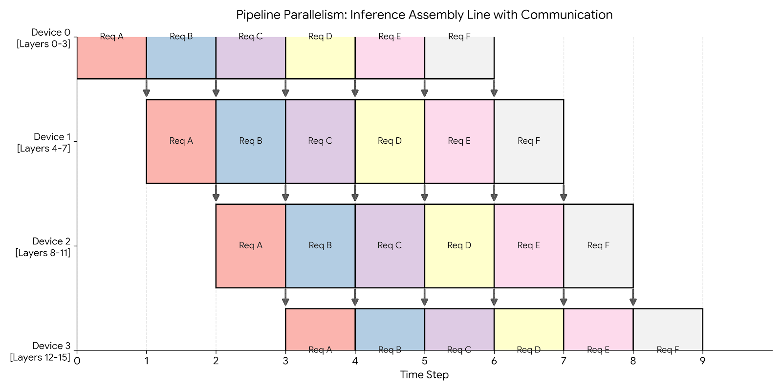
Inference
During inference, Pipeline Parallelism acts like a factory assembly line.
We can achieve 100% utilization by keeping the pipeline full. As soon as Device 0 finishes processing Request A and passes it to Device 1, it immediately picks up Request B. We fully overlap communication with computation.
Code for inference only using the Fake API
We run the same model as in Fake API but with an arbitrary amount of layers. This time, we have one layer per device. Device 0 will run layer 0. Device 1 will run ReLU and layer 1, etc. So even indices will run their layers only and odd indices will run ReLU and their layer. We implement the inference_loop to handle communicating the outputs of each layer.
class PipeliningInferenceOnly(ShardedEngine):
    def __init__(self, model_dim: int, hidden_dim: int):
        if self.device_id % 2 == 0:
            self.weights = np.zeros((model_dim, hidden_dim), dtype=np.float32)
        else:
            self.weights = np.zeros((hidden_dim, model_dim), dtype=np.float32)

    def load_checkpoint(self, params: dict[str, npt.ArrayLike]) -> None:
        # Load weights into local memory
        self.weights[...] = params[f'layers_{self.device_id}/weights'][...]

    def forward(self, x: npt.ArrayLike) -> npt.ArrayLike:
        # On odd layers (which receive hidden_dim), apply ReLU first
        if self.device_id % 2 != 0:
            x = relu(x)
        return np.einsum('bd,df->bf', x, self.weights)

    def inference_loop(self, input_stream: Reader[npt.ArrayLike], output_stream: Writer[npt.ArrayLike]) -> None:
        # LOGIC FOR DEVICE 0 (The Source)
        if self.device_id == 0:
            for x in iter(input_stream):
                out = self.forward(x)
                self.send(1, out)
        # LOGIC FOR OTHER DEVICES
        else:
            while True:
                # Block until we get data from the previous device
                x = self.receive(self.device_id - 1)
                out = self.forward(x)
                # If I am the last device, write to disk/network
                if self.device_id == self.num_devices - 1:
                    output_stream.write(out)
                else:
                    self.send(self.device_id + 1, out)
Training
Training is significantly harder due to the bidirectional dependency between the forward and backward pass.
- Forward Dependency: Layer
Nneeds input from LayerN-1. - Backward Dependency: Layer
N-1needs gradients from LayerN.
This creates a wait time known as the Pipeline Bubble.
- Idle Start: Device 3 sits idle waiting for the first data to propagate through Devices 0, 1, and 2.
- Idle End: Device 0 sits idle after its backward pass, waiting for the gradients to propagate back from Device 3.
Solution: Micro-batching To minimize the bubble, we split the global batch into smaller micro-batches. By processing smaller chunks, we can pass data to the next device sooner, allowing the pipeline to fill up faster.
Pros and cons
Pipelining is optimized for throughput (requests per second) at the cost of latency (time per request). It effectively uses multiple chips to simulate a single, massive chip.
| Feature | Impact | Why? |
|---|---|---|
| Throughput | ✅ High | During inference (or well-tuned training), all devices work in parallel. |
| Communication | ✅ Low | We only send activations between devices at the boundaries (e.g., after layer 4). This is much cheaper than Tensor Parallelism. |
| Latency | ❌ High | A single request must travel sequentially through all devices. Device 4 cannot start until Device 3 finishes. |
| Memory | ✅ Efficient | Parameters are split across devices, allowing us to fit larger models. |
Fully Sharded Data Parallel (FSDP)
With FSDP, not only do we shard the batch over multiple chips like with Data Parallelism, we also shard the optimizer state, the gradients and the parameters over multiple chips- This allows training models that are orders of magnitude larger than a single chip's memory.
Gather-Compute-Discard
The main mechanism behind FSDP is called Gather-Compute-Discard. Since parameters are sharded, a device cannot compute a layer immediately. It must first "borrow" the missing data from its neighbors.
- Shard: We initially fully shard tensors to reduce the per-chip memory.
- All-Gather (Weights): Before the forward pass of a layer, we All-Gather the parameters so that each chip momentarily holds a full replica of that specific layer.
- Compute: We compute the forward/backward pass with the full layer.
- Discard (Weights): We delete the parts of the tensor our chip did not initially owned to reduce memory requirements.
- Reduce-Scatter (Gradients): After the backward pass, instead of All-Reducing (which keeps a full copy of gradients everywhere), we Reduce-Scatter the gradients. Each chip ends up with only the specific chunk of gradients corresponding to the parameters it owns.
Note: The communication is typically overlapped with computation to hide latency.
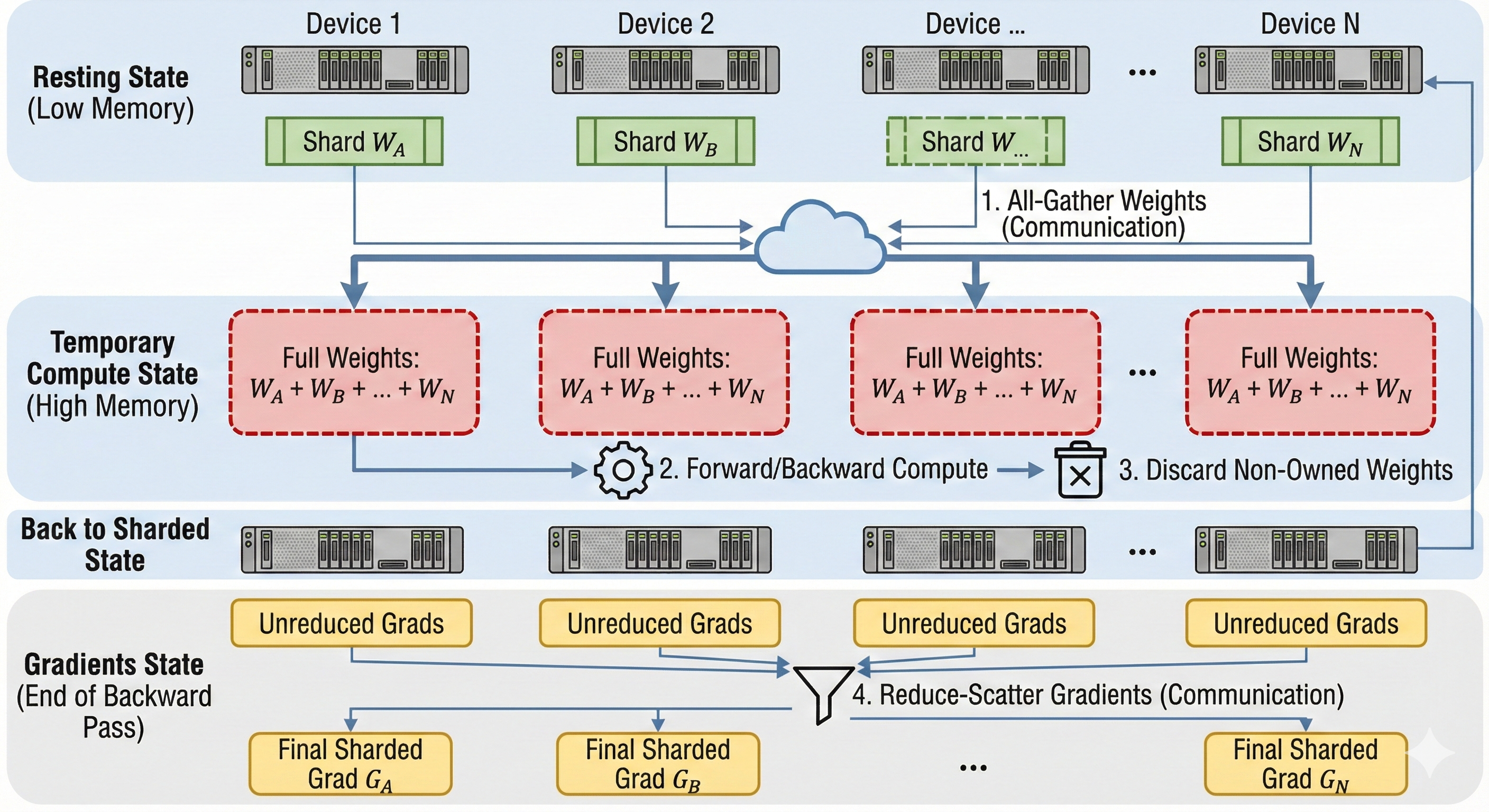
The three stages
Sharding more tensors means increasing the amount of All-Gathered data. Ideally we would shard as little as possible. Nonetheless, if only sharding the optimizer's state is not enough, we need to shard the gradients as well, or even the model parameters.
We often refer to the levels of sharding as the Three Stages of ZeRO, after Deepspeed's ZeRO paper.
| Stage | What is Sharded? | Memory Savings | Communication Overhead |
|---|---|---|---|
| ZeRO-1 | Optimizer States only | ~4x reduction. (Optimizer states are typically 75% of training memory). | Minimal (Same as DDP). |
| ZeRO-2 | Optimizer + Gradients | 8x reduction. | Minimal. |
| ZeRO-3 | Opt + Grads + Parameters | Linear reduction (\(1/N\)). Allows fitting massive models. | High. Requires All-Gather before every layer. |
Why is the optimizer state so large?
For every parameter, we hold:
- 2 bytes (bf16 weight)
- 2 bytes (bf16 gradient)
- 12 bytes (f32 optimizer state: master copy, momentum, variance)
Total: 16 bytes per parameter. Sharding just the optimizer states (12 bytes) removes 75% of the memory footprint without adding any extra communication steps (since All-Reduce and Reduce-Scatter transfer the same volume of data).
Pros and Cons
FSDP should only be used during training. It saves memory but doesn't speed up the math for a single sample; in fact, the communication overhead would make generation slower.
Code
Since our Fake API does not expose the optimizer's state, we will focus on sharding the model's weights and gradients.
To implement our initial unsharded model with FSDP, we need to change several things:
- Load a subset of the weights from our checkpoint.
- All-Gather the weights before each layer in the forward pass.
- Delete the gathered weights after using it (it would be implicit in an ML framework like Jax.)
- Reduce-Scatter the gradients after each layer of the backward pass.
Let's implement our 2 layers model with a ReLU activation, we shard the Model dimension across N devices such that each device holds Model/N:
- Correctness Note: We do not need to
Reduce-Scatterthe activations gradients, just the weights gradients. - Performance Note: In a production system, we would overlap the
All-Gatherfrom layerNwith the computations from layerN-1. We would also overlap theReduce-Scattersfrom layerN-1with the gradients computations from layerN.
class FSDP(ShardedEngine):

    def __init__(self, model_dim: int, hidden_dim: int):
        # How much data does a single device hold on the model axis
        self.local_model_dim = model_dim // self.num_devices

        self.w0 = np.zeros((self.local_model_dim, hidden_dim), dtype=np.float32)
        self.w1 = np.zeros((hidden_dim, self.local_model_dim), dtype=np.float32)
        # Context tape to store activations for backward pass
        self.activations = []


    def load_checkpoint(self, params: dict[str, npt.ArrayLike]) -> None:
        # Indices in the global array that belong to this device
        global_start_idx = self.device_id * self.local_model_dim
        global_end_idx = global_start_idx + self.local_model_dim

        # Load weights into local memory
        self.w0[...] = params['layer_0/weights'][global_start_idx:global_end_idx, :]
        self.w1[...] = params['layer_1/weights'][:, global_start_idx:global_end_idx]

    def forward(self, x: npt.ArrayLike) -> npt.ArrayLike:
        # -- Same as in single device --
        self.activations.append(x)

        # All-Gather w0
        w0_global = self.all_gather(self.w0, axis=0)

        # -- Same as in single device --
        z = np.einsum('bd,df->bf', x, w0_global)

        # Delete gathered data
        del w0_global

        # All-Gather w1
        w1_global = self.all_gather(self.w1, axis=1)

        # -- Same as in single device --
        self.activations.append(z)
        x = relu(z)
        out = np.einsum('bf,fd->bd', x, w1_global)

        # Delete gathered data
        del w1_global

        return out

    def backward(self, grads: npt.ArrayLike) -> dict[str, npt.ArrayLike]:
        """
        grads: Incoming gradient dL/d(Output) of shape (Batch, Model_Dim)
        """
        # -- Same as in single device --
        z = self.activations.pop()
        h_relu = relu(z)
        w1_grad = np.einsum('bf,bd->fd', h_relu, grads)

        # Reduce-Scatter w1_grad
        w1_grad = self.reduce_scatter(w1_grad, op='avg', axis=1)
        # All-Gather w1 again
        w1_global = self.all_gather(self.w1, axis=1)

        # -- Same as in single device --
        grads = np.einsum('bd,fd->bf', grads, w1_global)

        # Delete gathered weights
        del w1_global

        # -- Same as in single device --
        grads = grads * (z > 0)
        x_input = self.activations.pop()
        w0_grad = np.einsum('bd,bf->df', x_input, grads)

        # Reduce-Scatter w0_grad
        w0_grad = self.reduce_scatter(w0_grad, op='avg', axis=0)

        return {'layer_0/weights': w0_grad, 'layer_1/weights': w1_grad}
Tensor Parallelism (TP)
Tensor Parallelism shards the model's parameters and synchronizes the activations using collective operations. It allows saving on memory per chip while also lowering latency by splitting computations across multiple devices.
FSDP gathers the specific layer's parameters just in time for compute and discards them immediately after. The distinction is FSDP shards state (weights/optimizer), whereas TP shards computation (matrix multiplication).
There are multiple ways to implement Tensor Parallelism. The best method will depend on your model's architecture and dimensions. A common example for LLMs is Megatron Sharding.
How to think about TP?
The golden rule of TP is: Internal bandwidth is fast; Inter-chip bandwidth is slow. We want to structure our matrix multiplications so that we don't need to talk to other chips between every operation.
We achieve this by pairing two specific types of sharding:
- Column Parallelism (Layer 0 in the code example):
- Split the weight matrix \(W_0\) along the columns (Hidden Dimension).
- Input \(X\) is replicated.
- Each chip computes a chunk of the output vectors.
- Result: The output activation \(Z\) is sharded along the hidden dimension. No communication needed.
- Row Parallelism (Layer 1 in the code example):
- Split the weight matrix \(W_1\) along the rows (Hidden Dimension).
- Input \(Z\) is already sharded along the hidden dimension (thanks to Layer 0).
- Each chip computes a dot product using its local shard.
- Result: Each chip has a partial sum of the final output.
- Communication: We perform one single All-Reduce to sum the partial results.
By combining these, we perform an entire MLP block (Linear->ReLU->Linear) with only one synchronization step at the very end.
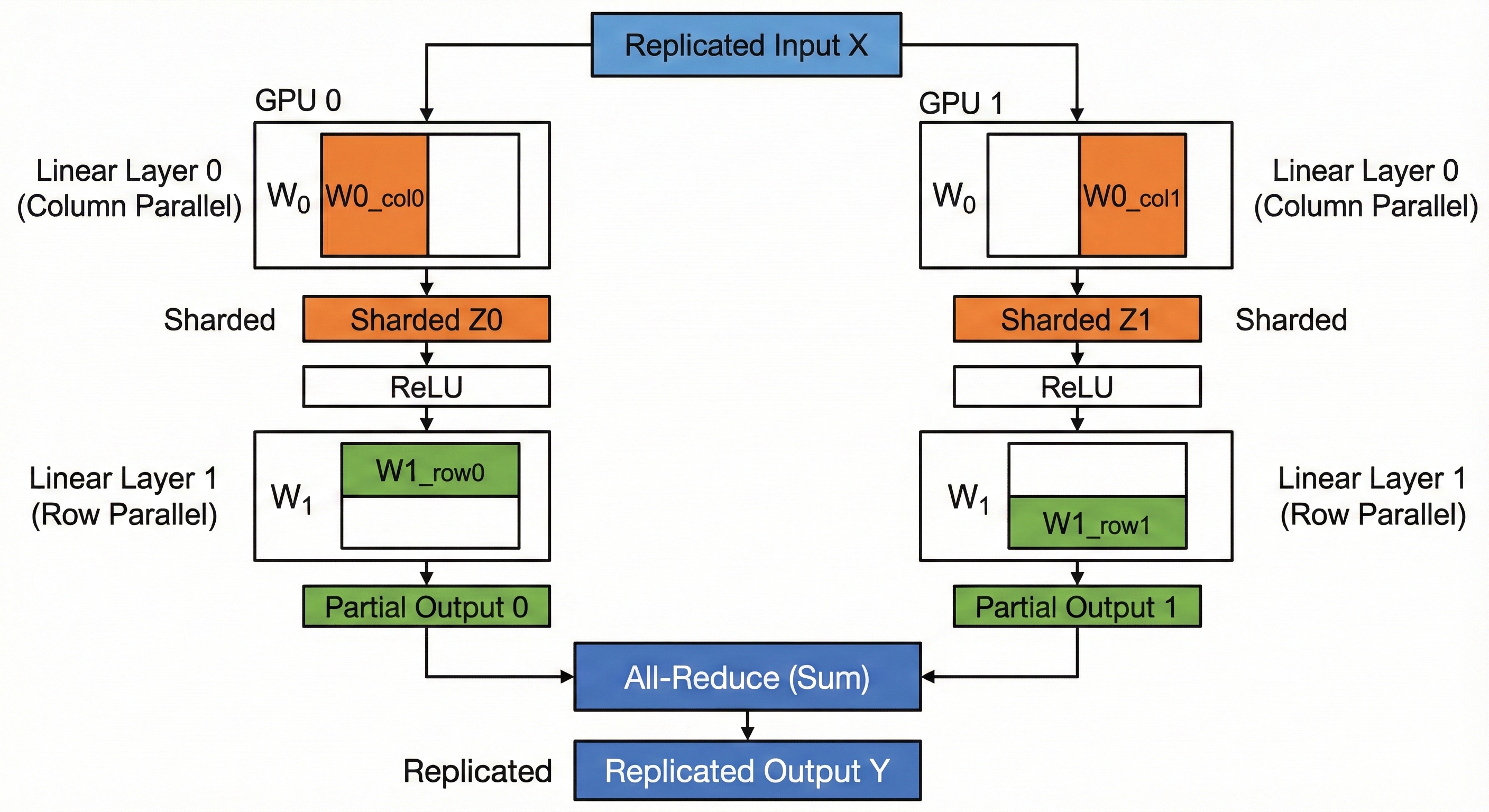
Code
Let's implement our initial unsharded model with Tensor Parallelism.
We implement the standard Megatron-style TP.
- World Size (N): Number of devices.
- \(W_0\): Shape \((Model, Hidden // N)\).
- \(W_1\): Shape \((Hidden // N, Model)\).
We assume the input x is replicated (identical copies on all devices).
class TensorParallel(ShardedEngine):

    def __init__(self, model_dim: int, hidden_dim: int):
        # We divide the Hidden dimension by the number of devices
        self.local_hidden_dim = hidden_dim // self.num_devices

        # W0: Column Parallel (Split output dim)
        self.w0 = np.zeros((model_dim, self.local_hidden_dim), dtype=np.float32)

        # W1: Row Parallel (Split input dim)
        self.w1 = np.zeros((self.local_hidden_dim, model_dim), dtype=np.float32)

        self.activations = []

    def load_checkpoint(self, params: dict[str, npt.ArrayLike]) -> None:
        # Determine which slice of the Hidden dimension this device owns
        start = self.device_id * self.local_hidden_dim
        end = start + self.local_hidden_dim

        # Load W0: Slice columns
        self.w0[...] = params['layer_0/weights'][:, start:end]

        # Load W1: Slice rows
        self.w1[...] = params['layer_1/weights'][start:end, :]

    def forward(self, x: npt.ArrayLike) -> npt.ArrayLike:
        # x is Replicated: Shape (Batch, Model)
        self.activations.append(x)

        # 1. Column Parallel Linear
        # (Batch, Model) @ (Model, Hidden/N) -> (Batch, Hidden/N)
        # Each device computes a valid slice of the output vector.
        z = np.einsum('bd,df->bf', x, self.w0)

        # NO COMMUNICATION NEEDED HERE
        # The output 'z' is inherently sharded along the Hidden axis.

        # 2. Activation
        # ReLU works element-wise, so we can apply it to the shards independently.
        self.activations.append(z)
        z = relu(z)

        # 3. Row Parallel Linear
        # (Batch, Hidden/N) @ (Hidden/N, Model) -> (Batch, Model)
        # We contract the sharded axis (Hidden).
        # This results in a PARTIAL SUM of the output.
        partial_out = np.einsum('bf,fd->bd', z, self.w1)

        # 4. All-Reduce
        # Sum the partial results from all devices to get the final full output.
        out = self.all_reduce(partial_out, op='sum')

        return out

    def backward(self, grads: npt.ArrayLike) -> dict[str, npt.ArrayLike]:
        """
        grads: Incoming gradient dL/d(Output) of shape (Batch, Model)
        """
        # --- Backprop Layer 1 (Row Parallel) ---
        # The forward pass ended with an All-Reduce (Sum).
        # The backward pass of All-Reduce(Sum) is Identity (copy gradients to all).
        # So 'grads' is already correct and replicated.

        z = self.activations.pop() # Shape (Batch, Hidden/N)
        h_relu = relu(z)

        # dL/dW1 = h.T @ grads
        # (Hidden/N, Batch) @ (Batch, Model) -> (Hidden/N, Model)
        # Result matches local W1 shape. No comms needed.
        w1_grad = np.einsum('bf,bd->fd', h_relu, grads)

        # dL/dz = grads @ W1.T
        # (Batch, Model) @ (Model, Hidden/N) -> (Batch, Hidden/N)
        # Result is sharded (matches z). No comms needed.
        dz = np.einsum('bd,fd->bf', grads, self.w1)

        # --- Backprop Layer 0 (Column Parallel) ---
        dz = dz * (z > 0) # Backprop ReLU
        x_input = self.activations.pop() # Shape (Batch, Model)

        # dL/dW0 = x.T @ dz
        # (Model, Batch) @ (Batch, Hidden/N) -> (Model, Hidden/N)
        # Result matches local W0 shape. No comms needed.
        w0_grad = np.einsum('bd,bf->df', x_input, dz)

        # dL/dx = dz @ W0.T
        # (Batch, Hidden/N) @ (Hidden/N, Model) -> (Batch, Model)
        # We are contracting the sharded axis (Hidden/N).
        # This produces a PARTIAL SUM of dx.
        dx_partial = np.einsum('bf,df->bd', dz, self.w0)

        # To get the true dL/dx, we would need to All-Reduce here.
        # However, for weight updates, we strictly return the weight gradients below.

        return {'layer_0/weights': w0_grad, 'layer_1/weights': w1_grad}
Practice Questions
A Practical Example
Let's explore a simple example of a post attention projection.
batch = 256
length = 1024
d_model = 4096
num_heads = 16
key_size = d_model // num_heads

# B L N K
x = torch.rand((batch, length, num_heads, key_size), dtype=torch.bfloat16, device='cuda')

# N K D
w = torch.rand((num_heads, key_size, d_model), dtype=torch.bfloat16, device='cuda')

out = torch.einsum('blnk,nkd->bld', x, w)
- How would pipelining work here (assuming multiple layers)?
- How would data parallelism work?
- What different ways can we implement tensor parallelism?
- How would we implement FSDP?
LLM Serving Optimizations
This chapter covers an array of optimization techniques that are frequently used when serving LLMs. Some of these techniques can be applied to other types of models, and some can also be applied to training (for instance flash attention). We subdivide the techniques into two sub-parts: Quality Neutral and Quality Detrimental. Quality Neutral techniques improve latency or throughput without deteriorating the quality of the output while Quality Detrimental techniques have a negative impact on the quality of the model; they offer a tradeoff between latency and quality.
Quality Neutral
Quality Neutral optimization techniques should almost always be used as they make inference much faster and cheaper without any degradation on the model's output. Unfortunately, these techniques require more work to implement than the Quality Detrimental ones.
It is important to understand KV caching before disaggregated serving because the later builds on the former.
KV Caching
KV Caching is one of the most fundamental optimization techniques for LLMs. It trades off memory for latency by caching the \(K\) and \(V\) activations.
Let's take a look at this small stripped down implementation of the attention mechanism. In the einsums we have:
- \(s=sequence\_length_q\)
- \(t=sequence\_length_k\)
- \(d=model\_dim\)
- \(n=num\_heads\)
- \(h=head\_dim\)
q = np.einsum('sd,dnh->snh', x, q_weights)
k = np.einsum('sd,dnh->snh', x, k_weights)
v = np.einsum('sd,dnh->snh', x, v_weights)

qk = np.einsum('snh,tnh->snt', q, k)
scores = softmax(qk, axis=-1)
out = np.einsum('snt,tnh->snh', scores, v)
When we first pass the tokens through our model, we need to execute this full computation. The \(Q@K^T\) part has quadratic complexity with regard to the sequence length (\(O(n^2)\).)
This first pass generates a single token. To get the next token after that, we need to add back the token we just created to the sequence (\(x\) here), and rerun the whole model again. We do this in a loop until we reach a special <end> token.
However, we notice that a lot of this work is redundant after the first step. First of all, we do not need to multiply each token in \(q\) again, just the one we produced in the previous step, this makes the complexity per step \(O(n)\) where \(n\) is the current sequence length.
Furthermore, we can just cache the previous \(k\) and \(v\) projections so we do not have to recompute them fully at each step. We once again only project the last produced token. This would otherwise be prohibitively expensive for large sequence lengths.
We typically call the first step with a large sequence length Prefill and the subsequent steps that process a single token Decode.
Here is some pseudcode to show how decode would be implemented:
# Notice that we only attend to a single token
q_current = np.einsum('1d,dnh->1nh', x[-1:], q_weights)
k_current = np.einsum('1d,dnh->1nh', x[-1:], k_weights)
v_current = np.einsum('1d,dnh->1nh', x[-1:], v_weights)

# Store the new activations
kv_store.append(k_current, v_current)

# Get the full kv cache
k, v = kv_store.get()

# q_current @ k^T
# Attention: Compare current query (1) against all keys (t)
# Note: 't' grows by 1 at every step
qk = np.einsum('1nh,tnh->1nt', q_current, k)
scores = softmax(qk, axis=-1)
out = np.einsum('1nt,tnh->1nh', scores, v)
This approach raises a new problem of its own. The Prefill step is compute-bound, we have a large sequence to which we apply a quadratic matrix multiplication. On the flip side, the Decode steps are memory bound, they operate on a small batch size of 1. This is exacerbated in the MLP layers. Since we are only processing a single token (Batch Size = 1), we have to retrieve the entire, massive weight matrix from memory just to perform a single matrix-vector multiplication. We spend more time moving data than computing.
Thankfully, there is a solution for this in the next chapter on Disaggregated Serving.
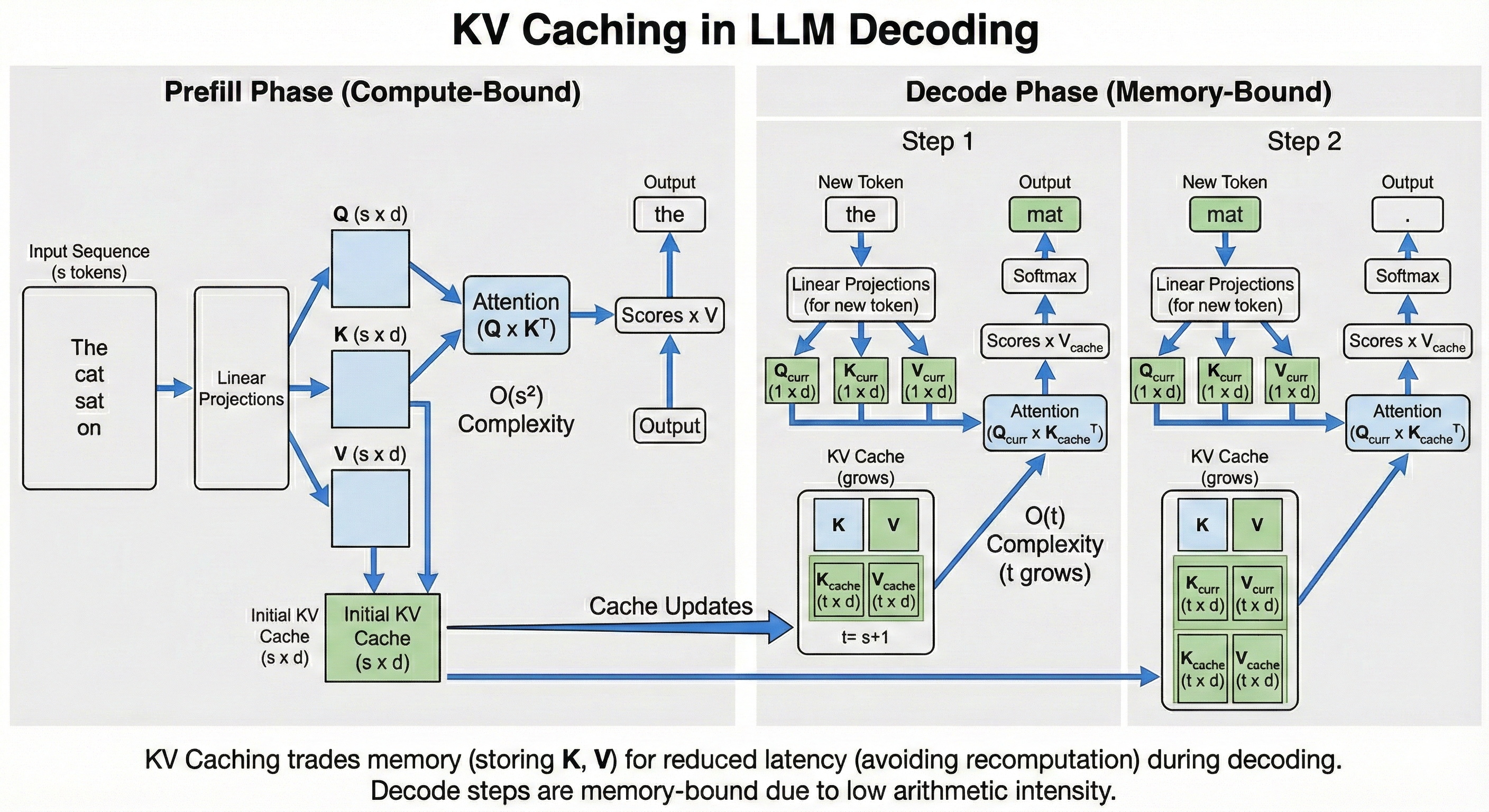
Disaggregated Serving
As discussed in the previous chapter on KV Caching, LLM generation is split into two phases:
Prefillinitiallly processes the full sequence length with quadratic complexity and produces the originalKV Cacheas well as the first output token.Prefillis usually compute bound.Decodeis called repeatedly in a loop until we reach an<end>token, it only processses the last token that was generated in the previous step. Since it only processes a single token at a time,Decodesteps are largely memory bound.
While a single Decode step is usually multiple orders of magnitude faster than Prefill, we actually spend the majority of our time in the Decode loop because we have to perform so many steps.
We end up with two pretty different compute regimen, even though we are processing the same model with the same weights and equations.
One solution would be to simply increase the batch size, instead of processing a single sequence at a time, we could process 64 in parallel for instance. This would help make Decode compute bound. However, processing 64 Prefill at once would increase the latency of the first tokens we stream back to our clients 64 times (since we are already compute bound in Prefill), which would be unacceptable.
The Solution: Disaggregated Serving
We want a large batch size in Decode to make it compute bound. We want a small batch size (usually 1 sequence at a time) in Prefill to keep the user's latency low (Time to First Token).
The solution is Disaggregated Serving: separating the model into two distinct pools of workers.
- Prefill Instances: Optimized for compute. They take a request, process the prompt, and generate the initial KV Cache.
- Decode Instances: Optimized for memory bandwidth. They take the initialized state and stream the rest of the tokens.
How it works
For instance, we can run a single Decode server with batch size 64, and two Prefill servers with batch size 1.
- The
Prefillserver processes a prompt and computes the initial KV Cache. - KV Transfer: This is the critical step. The Prefill server sends the computed KV Cache (which can be Gigabytes of data) over the network to the
Decodeserver. - The
Decodeserver loads this cache into its memory and adds the request to its running batch loop.
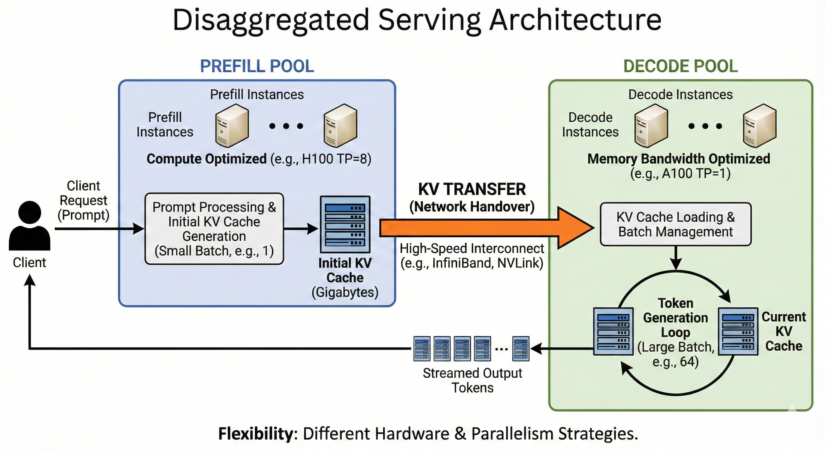
Topology and Hardware Flexibility
Because we have decoupled the phases, we are no longer forced to use the same hardware or parallelism strategies for both. We can "right-size" our infrastructure:
- Different Chip Counts (Tensor Parallelism):
- Prefill: We might shard the model across 8 GPUs (TP=8). Since we have a massive amount of computation to do, splitting the work across 8 chips divides the latency by roughly 8. This is crucial for user responsiveness.
- Decode: If we sharded the same way here, we would be waiting on network communication (All-Reduce) just to generate a few tokens. We usually favor Data Parallelism (running multiple independent copies of the model) over Tensor Parallelism. Since decoding is memory-bound, we don't need to split the compute across chips to go faster; we prefer to avoid the communication overhead of sharding.
- Different Architectures:
- Prefill: We can use compute-dense chips (e.g., NVIDIA H100) to crunch the prompt as fast as possible.
- Decode: We can use older, cheaper chips with high memory bandwidth (e.g., A100s) or even specialized inference chips, as we just need to hold the KV cache and move it to the compute units quickly.
The Trade-off: KV Transfer
There is no free lunch. The cost of this architecture is the Network Handover.
When the Prefill server finishes, the KV Cache resides in its HBM (GPU Memory). To start decoding on a different server, we must transmit this cache over the network. For long sequences, this can be Gigabytes of data.
To make this viable, we usually need high-speed interconnects (like InfiniBand or NVLink) to ensure the time spent sending the data doesn't outweigh the time saved by splitting the workload.
Speculative Decoding
What if instead of generating one token at a time in Decode, we could generate multiple? This is the premise of Speculative Decoding.
This paper observes that most tokens are relatively easy to predict. For instance the sentence, In Rome, I was eating a piz, the next token is very easy to predict as za. We do not need a massive model to predict it. So instead, let's use a smaller, less capable, but much faster model to predict easy tokens and have the large model intervene for the harder ones.
How it works
We call the small model the Drafter and the large model the Verifier.
We first have to pick an existing small model, or train a Drafter to aproximate the distribution of the Verifier model with a much smaller number of parameters.
Then during inference, before each Verifier step, we first run multiple steps of the Drafter, for instance 4, we call this number \(\gamma\). Then, we add the \(\gamma\) generated tokens to the Verifier's input and we run them through the model in parallel.
At the end, we loop over the distributions of each output token.
- We compare the probability distribution of the
Drafteragainst theVerifier. If the token drawn by theDrafteris plausible enough according to the Verifier, we accept it. - Otherwise, we reject the token and resample it with an adjusted distribution \(p'(x) = norm(max(0, p_{verifier}(x) - p_{drafter}(x)))\). We stop here and reject the rest of the predicted tokens.
- If we accepted all tokens, we use the model's last prediction.
This means that if we set \(\gamma = 4\), each step might generate between 1 and 5 tokens.
Mathematical Intuition
The formula for accepting a token is \[\text{is_accepted} = \text{random_uniform}(0, 1) < \frac{P_{\text{verifier}}(x)}{P_{\text{drafter}}(x)}\]
If the Verifier thinks the token is more likely than the Drafter did, we always accept. If it thinks it's less likely, we accept or reject probabilistically.
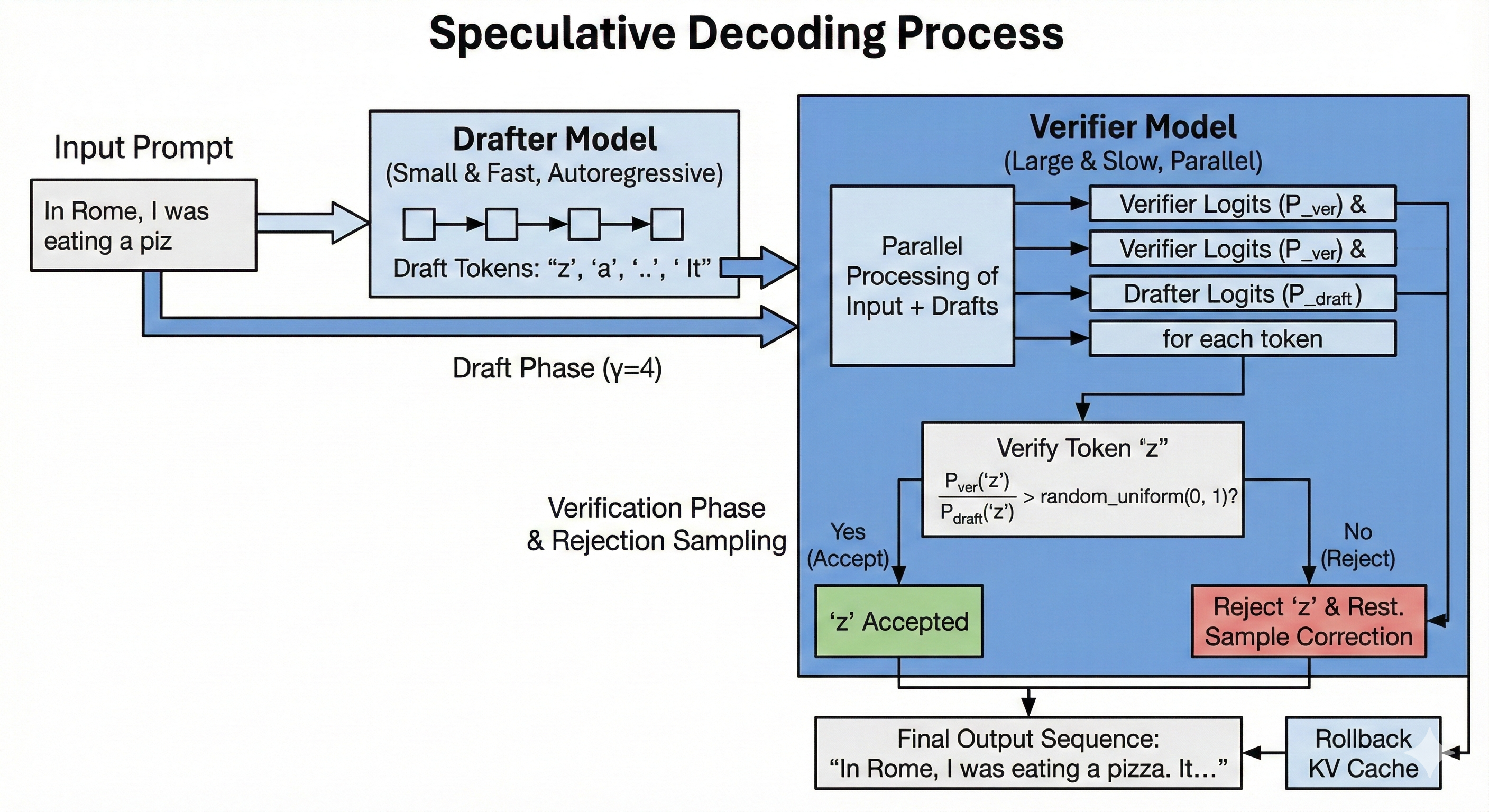
Pseudocode
gamma = 4

# NOTE: The Verifier must manage a KV Cache that can be 'rolled back'
kv_state = verifier.prefill(inputs)

# 1. Draft Phase (Sequential)
draft_tokens = []
for _ in range(gamma):
    # The drafter runs autoregressively
    token = drafter.generate_one(kv_state + draft_tokens)
    draft_tokens.append(token)

# 2. Verification Phase (Parallel)
# The verifier processes the original input + all drafts at once
# Returns logits for positions: [last_input, d1, d2, d3, ...]
verifier_logits = verifier.forward(kv_state + draft_tokens)

accepted_tokens = []
for i, draft_token in enumerate(draft_tokens):
    # Get probabilities for the specific token 'draft_token'
    p_ver = prob(verifier_logits[i], draft_token)
    p_draft = prob(drafter_logits[i], draft_token)

    # Rejection Sampling Formula
    # Accept if Verifier is confident, or probabilistically otherwise
    if np.random.random() < (p_ver / p_draft):
        accepted_tokens.append(draft_token)
    else:
        # Rejection! Sample a correction from the residual distribution
        # (p_ver - p_draft) re-normalized
        correct_token = sample_correction(verifier_logits[i], p_draft)
        accepted_tokens.append(correct_token)
        break # Stop accepting drafts
else:
    # Bonus token: If all drafts accepted, we get one extra token "for free"
    extra_token = sample(verifier_logits[-1])
    accepted_tokens.append(extra_token)

# 3. Rollback / Pruning
# The verifier.forward() call above computed KV entries for ALL draft tokens.
# If we rejected early, the cache now contains invalid future states.
# We must truncate the Verifier's KV Cache to keep only the valid prefix.
verifier.rollback(keep_tokens=len(accepted_tokens))

# Append valid tokens to state
kv_state.append(accepted_tokens)
The Added Latency Paradox
An interesting byproduct of this method is that each individual step is becoming slower. We have to first run multiple steps of the Drafter, then decode multiple tokens in parallel using the Verifier.
The added latency from the Drafter can be managed by keeping the Drafter small. The added tokens to the Verifier do not add a lot of latency because we are so much memory bound in Decode anyway.
We reduce latency not by making each step faster, steps are actually longer. We reduce latency by increasing the total amount of tokens generated at every step. If the Drafter is good enough, it can significantly reduce overall latency.
In production, we need to monitor the impact on step time of the technique as well as the average amount of tokens accepted per step. These two data points will inform how we should set \(\gamma\).
- If the average accepted tokens count is
3, but \(\gamma=10\). We clearly should reduce \(\gamma\) to around4. - On the other hand, if we accept nearly all tokens, we should consider increasing \(\gamma\).
Lenience
So far, Speculative Decoding is a quality neutral technique. However, the authors of the paper introduced a lesser known component in the appendix: lenience.
It simply changes the acceptance formula to
\[\text{is_accepted} = \text{random_uniform}(0, 1) < \frac{P_{\text{verifier}}(x)}{P_{\text{drafter}}(x) * lenience}\]
It is another knob we can turn to increase the amount of predicted tokens artificially. The lower the value, the more tokens we accept. However, this means that we are now accepting tokens we normally would not have. It is mostly fine because we still reject tokens that make no sense at all (depending on the lenience value.) Lenience should be empirically tested before applying. A nice property is that it can simply be set dynamically during serving, so during traffic spikes, the value could be lowered, thus reducing latency.
Flash Attention
The main bottleneck of the attention mechanism comes from the softmax in the attention scores computation.
scores = softmax(np.einsum('btnh,bsnh->btns', q, k))
out = np.einsum('btns,bsnh->btnh', scores, v)
The size of the scores tensor scales quadratically with regard to the sequence length \(O(sequence\_length ^ 2)\). Because we apply softmax to the output, we materialize the whole intermediate array. We very quickly run out of memory to store this intermediate array when reaching large batch sizes.
Furthermore, the naive implementation reads the \(QK^T\) product twice from HBM:
- Compute the sum of the exponentials \(\sum_{j=1}^{n} \exp{x_j}\)
- Apply \(softmax(x_i) = \frac{\exp{x_i}}{\sum_{j=1}^{n} \exp{x_j}} \)
Flash Attention solves the memory issue and reduces the amount of memory to read by introducing the Online Softmax trick.
Instead of materializing the whole array, summing it, and dividing each value; we split \(Q\), \(K\), and \(V\) into sub-blocks and we compute the attention block by block. Since the softmax needs to know about the full sequence, we need to reconcile the values across blocks, we do this by keeping a state. Specifically:
- \(m = max(S_i)\). The maximum value. Used to prevent overflowing.
- \(\ell = \sum{\exp(S_i - m_i)}\). Normalization denominator for
softmax.
For each block, softmax becomes:
\[\text{softmax}(S_i) = \frac{e^{S_i - m}}{\ell}\]
The Update Rule: When merging a new block \(j\) with our running state, we update the output \(O\) as:
\[O_{new} = \text{diag}(\ell_{new})^{-1} (\text{diag}(\ell_{old})e^{m_{old} - m_{new}} O_{old} + e^{m_{j} - m_{new}} P_{j} V_{j})\]
This is scary, but it's simply the line:
O_block = (O_block * old_scale) + (new_scale * (P_ij @ V_block))
IO Complexity
Standard attention requires \(O(N^2)\) HBM accesses (to read/write the huge attention matrix). Flash Attention reduces this memory access significantly by keeping intermediate results in SRAM, though the computational complexity (FLOPs) remains quadratic.
Code
We implement a minimal flash attention function in numpy. The goal is to illustrate the general logic.
Note that we would typically write a CUDA or Pallas kernel to run on a GPU or TPU. And the shape should be (batch,seq_len,num_head,head_dim) instead of (seq_len,d_model).
def flash_attention(Q, K, V, block_size=64):
    N, d = Q.shape
    scale = 1 / np.sqrt(d)

    # Initialize output
    O = np.zeros((N, d))

    # Divide Q into blocks (Rows)
    # The Outer Loop loads a block of Queries from HBM to SRAM
    for i in range(0, N, block_size):
        i_end = min(i + block_size, N)
        Q_block = Q[i:i_end, :]    # Shape: (Br, d)

        # Initialize running stats for THIS block of rows
        # shape: (Br, 1)
        m = np.full((i_end - i, 1), -np.inf)
        l = np.zeros((i_end - i, 1))

        # Current accumulator for this block of rows
        O_block = np.zeros((i_end - i, d))

        # Divide K, V into blocks (Columns)
        # The Inner Loop loads blocks of K and V from HBM to SRAM
        for j in range(0, N, block_size):
            j_end = min(j + block_size, N)
            K_block = K[j:j_end, :] # Shape: (Bc, d)
            V_block = V[j:j_end, :] # Shape: (Bc, d)

            # --- 1. Compute Attention Scores for this sub-block ---
            # S shape: (Br, Bc)
            S_ij = (Q_block @ K_block.T) * scale

            # --- 2. Compute local stats for this sub-block ---
            m_ij = np.max(S_ij, axis=-1, keepdims=True) # Max of current block
            P_ij = np.exp(S_ij - m_ij)                  # Exponentials
            l_ij = np.sum(P_ij, axis=-1, keepdims=True) # Sum of curr block

            # --- 3. Update Global Stats (Online Softmax) ---
            # New max is max of old running max and current block max
            m_new = np.maximum(m, m_ij)

            # Correction factors
            # How much to shrink the old accumulator
            old_scale = np.exp(m - m_new)
            # How much to shrink the new block
            new_scale = np.exp(m_ij - m_new)

            # Update running sum l
            l = (l * old_scale) + (l_ij * new_scale)

            # Update Output Accumulator
            # O_new = O_old * scale_old + V_block * P_ij * scale_new
            O_block = (O_block * old_scale) + (new_scale * (P_ij @ V_block))

            # Update running max
            m = m_new

        # Finalize the block output and write to HBM
        O[i:i_end, :] = O_block / l

    return O
Validating
def standard_attention(Q, K, V):
    N, d = Q.shape
    scale = 1 / np.sqrt(d)

    # 1. Compute full scores matrix (N x N) - Memory intensive part!
    S = np.einsum('td,sd->ts', Q, K) * scale

    # 2. Compute max for numerical stability
    m = np.max(S, axis=-1, keepdims=True)

    # 3. Compute Softmax
    P = np.exp(S - m)
    l = np.sum(P, axis=-1, keepdims=True)
    P_norm = P / l

    # 4. Compute Output
    O = np.einsum('ts,sd->td', P_norm, V)

    return O

seq_len = 1024  # Sequence length
d = 64    # Head dimension
np.random.seed(42)

# Random Inputs
Q = np.random.randn(seq_len, d)
K = np.random.randn(seq_len, d)
V = np.random.randn(seq_len, d)

O_std = standard_attention(Q, K, V)
O_flash = flash_attention(Q, K, V, block_size=128)

# Compare
diff = np.abs(O_std - O_flash)
print(f"Max difference: {np.max(diff):.6e}")
print(f"Mean difference: {np.mean(diff):.6e}")
Quality Detrimental
Quality Detrimental optimization techniques lower the latency and the cost of serving the model but they also lower the quality of the model's output. One should be mindful when applying these methods and carefully analyze the cost to degradation ratio.
Quantization
We typically store a model's weights in the bfloat16 floating-point format. Which means that each parameter takes 2 bytes.
We can halve the memory bandwidth usage by simply using fp8 formats. We can even go further with smaller formats like int4 quantization all the way down to 1.58 bits quantization.
Hardware Support
Quantization is particularly useful in memory-bound regimens because it drastically reduces the amount of data movements. Besides, modern chips now support lower precision arithmetic with higher flops per second than with higher precision.
For instance, according to this, H100 GPUs can do 1979 teraFLOPS in bf16 while they can do 3958 teraFLOPS in fp8.
Note that there are no mentions of int4 in the table. This is because int4 is not hardware supported by the H100, so there would need to be a conversion to fp8 before using the tensor core. Therefore, int4 would not yield compute throughput gains, only bandwidth gains. It is important to check your hardware's specification.
Scales
Simply rounding weights to the nearest integer would degrade performance too much because model weights can have very different magnitudes (e.g., outliers). To solve this, we introduce a new tensor called scales.
The scales map the small integer range (e.g., -127 to 127) back to the original floating point range. A quantized dot product between activations \(x\) and quantized weights \(W_{quantized}\) with scales \(S\) looks like this: \[(x\cdot W_{quantized}) \times S\]
We first apply the matrix multiplication between \(x\) and \(W_{quantized}\) using the smaller dtype (fast), then we scale up the result using an element-wise product with \(S\) in the original dtype but with a much smaller tensor.
If the original weights had a shape of (d_in, d_out), the scales typically have a shape of (1, d_out). This is called Channel-wise Quantization. The scales are tiny compared to the weights, adding negligible memory overhead.
Obtaining the Quantized Weights and Scales
There are different methods of obtaining the weights and scales. A simple and common approach is called Symmetric Block-wise Quantization. We map the absolute maximum value of a row/column to the maximum integer value (e.g., 127 for int8).
- Calculate the absolute maximum value for the channel: \(\alpha = \max(|W|)\).
- Calculate the Scale (\(S\)): \(S = \frac{\alpha}{127}\).
- Calculate Quantized Weights (\(W_{quantized}\)): \(W_{quantized} = \text{round}(\frac{W}{S})\)
- Dequantization (Forward Pass): \(\text{output} = (x @ W_{quantized}) \times S\)
Code Example
import numpy as np

# 1. Create random weights in float16
# Shape: (Input Dim, Output Dim)
d_in, d_out = 64, 128
weights = np.random.normal(size=(d_in, d_out)).astype(np.float16)

# 2. Calculate Scales (Channel-wise)
# We want one scale per output column -> Shape (1, d_out)
# We use int8, so max_int is 127
max_val = np.max(np.abs(weights), axis=0, keepdims=True)
scales = max_val / 127.0

# 3. Quantize
# Divide, Round, and Cast to int8
weights_quantized = (weights / scales).round().astype(np.int8)

print(f"Original Memory: {weights.nbytes} bytes")
print(f"Quantized Memory: {weights_quantized.nbytes + scales.nbytes} bytes")

# 4. Dequantization (Forward Pass)
# We simulate the matmul. In reality, hardware does this in mixed precision.
x = np.random.randn(1, d_in).astype(np.float16)

# Integer Matmul
out_int = x @ weights_quantized

# Rescale to float
out_float = out_int * scales
Mixture of Experts (MoE)
Mixture of Experts (MoE henceforth) is arguably the most impactful modeling innovation since the attention mechanism. It allows increasing the number of parameters in the MLP block without proportionally increasing the number of flops.
Instead of a single large matrix multiplication, we split our weights into \(e\) experts. Each token gets assigned to \(k\) experts based on a router (which is learnt.) We train \(e\) experts but only activate \(k\) experts per token during inference.
In the next sub-chapters, we will implement a simple kernel for single device MoE, then we will discuss different sharding strategies, and discuss problems with inefficient load balancing (expert imbalance.) For now, let's implement a NumPy version of MoE.
Basic Implementation
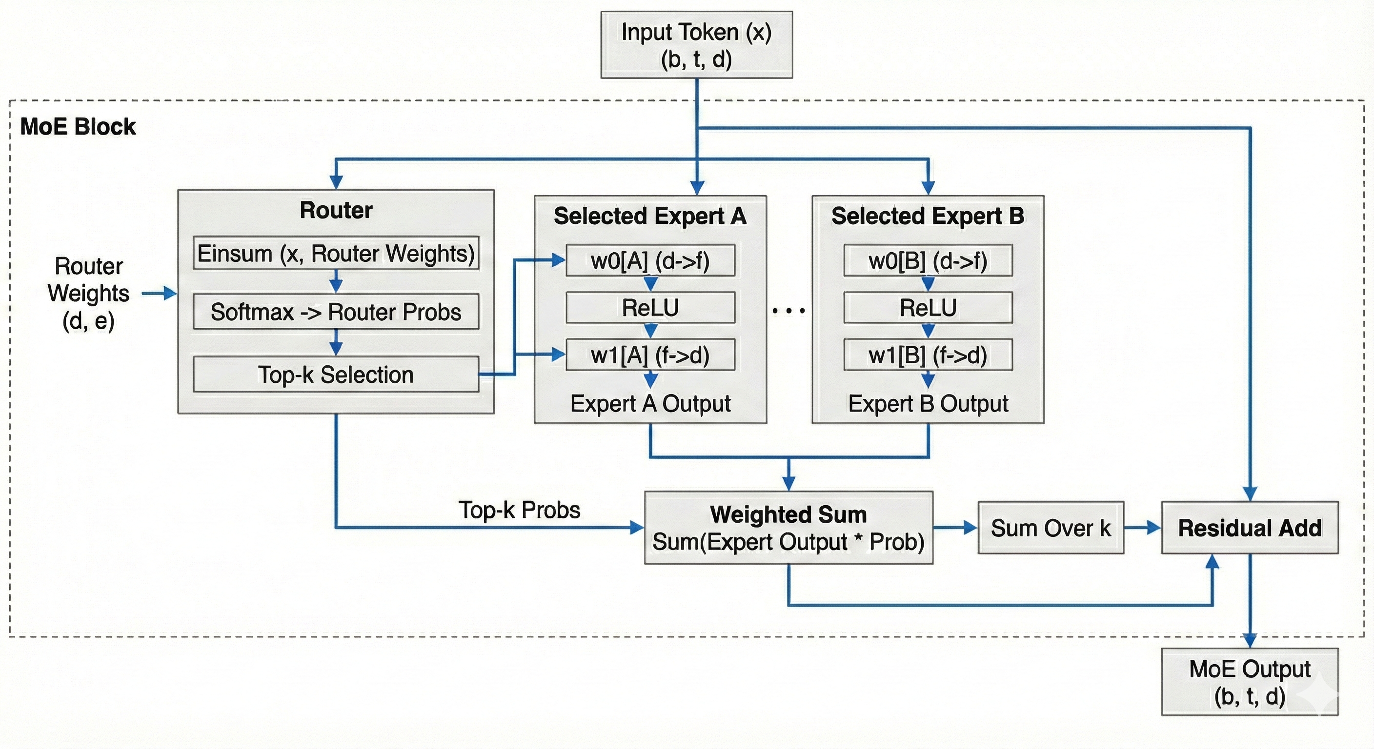
import numpy as np

def softmax(x):
    e_x = np.exp(x - np.max(x, axis=-1, keepdims=True))
    return e_x / np.sum(e_x, axis=-1, keepdims=True)

def moe(x, router_weights, w0, w1, k: int = 2):
    """
    x: (b, t, d)
    router_weights: (d, e)
    w0: (e, d, f)
    w1: (e, f, d)
    """
    num_experts = w0.shape[0]
    b, t = x.shape[:2]

    # (b, t, d) -> (bt, d)
    x = x.reshape(-1, x.shape[-1])

    expert_choices = np.einsum('Bd,de->Be', x, router_weights)
    # (bt, e)
    router_probs = softmax(expert_choices)
    # Indices of the top k experts
    # (bt, k)
    top_k_indices = expert_choices.argsort(axis=-1)[..., -k:]

    # Probabilities corresponding to those experts
    # (bt, k)
    top_k_probs = np.take_along_axis(router_probs, top_k_indices, axis=-1)

    # Normalize
    top_k_probs /= top_k_probs.sum(axis=1)

    # Assign tokens to experts
    tokens_to_expert = [[] for _ in range(num_experts)]
    # Store the mapping to reconstruct order later: (expert_id, original_token_idx, k_rank)
    reorder_map = [[] for _ in range(num_experts)]

    for token_idx, expert_ids in enumerate(top_k_indices):
        for k_rank, expert_id in enumerate(expert_ids):
            tokens_to_expert[expert_id].append(x[token_idx][None, ...])
            reorder_map[expert_id].append((token_idx, k_rank))

    # Placeholder for the final combined output
    # (bt, k, d)
    expert_outputs = np.zeros((x.shape[0], k, d))
    # Apply dot products to each expert
    for expert_idx in range(num_experts):
        if not tokens_to_expert[expert_idx]:
            continue
        tokens = np.concatenate(tokens_to_expert[expert_idx])
        # w0
        y = np.einsum('Bd,df->Bf', tokens, w0[expert_idx])
        # relu
        y = np.maximum(y, 0)
        # linear
        y = np.einsum('Bf,fd->Bd', y, w1[expert_idx])
        for i, (token_idx, k_rank) in enumerate(reorder_map[expert_idx]):
            expert_outputs[token_idx, k_rank] = y[i]

    # Multiply expert output by router probability
    # expert_outputs: (bt, k, d)
    # top_k_probs: (bt, k) -> broadcast to (bt, k, 1)
    weighted_out = expert_outputs * top_k_probs[:, :, None]

    # Reduce over k. Different papers use different methods
    # (bt, d)
    out = weighted_out.sum(axis=1)
    # (b, t, d)
    out = out.reshape(b, t, -1)
    # Residual
    return out + x.reshape(b, t, -1)
Expert Sharding
MoE opens the door to a new sharding strategy: Expert Sharding. We assign experts to different devices, after we compute the expert choices, we send the tokens to the correct devices where we perform the computations. We then send them back to where they came from.
It is quite different to other sharding strategies because each device will see a different set of tokens and will compute a different amount of tokens.
The only difference with the basic single device implementation is that instead of appending to the local list, we send the tokens to the device who hold the correct experts. The difficulty is that the amount we send to each device is dynamic. Typically, we will need to communicate to each other device in the mesh how many tokens we are sending them. This means we need to All-To-All some metadata about how many tokens were sent from each device concurrently to the tokens we are sending.
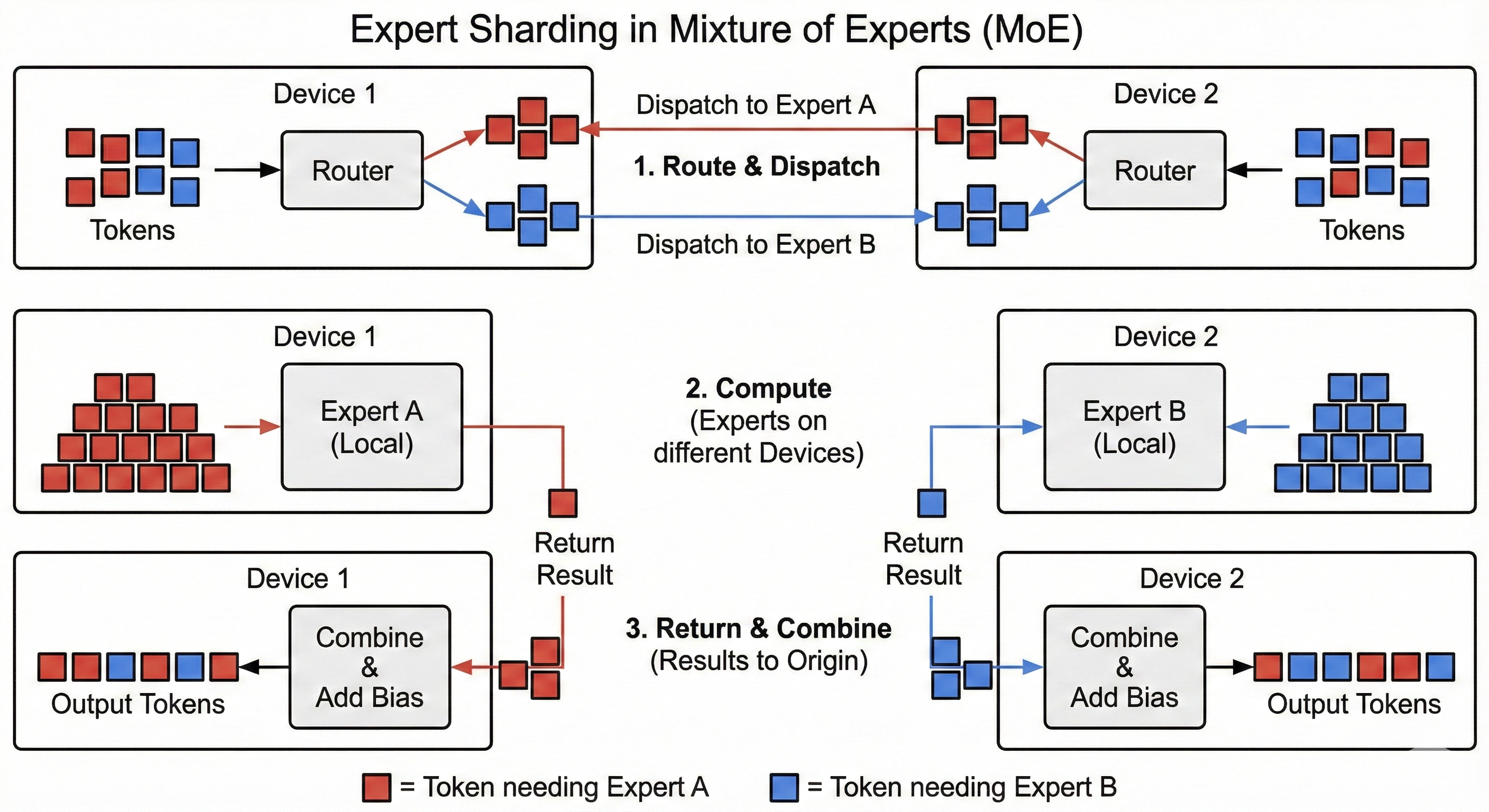
Let's rewrite the code using the same Pseudo API using the logic you would find in an MoE kernel but with simplified APIs.
...

def forward(self, x, router_weights, w0, w1, k: int = 2):
    """
    x: (b_per_device, t, d)
    router_weights: (d, e_total)
    w0: (e_per_device, d, f)
    w1: (e_per_device, f, d)
    """
    num_experts_total = router_weights.shape[1]
    num_experts_per_device = w0.shape[0]

    # -- SAME AS SINGLE DEVICE --
    b, t, d = x.shape
    x = x.reshape(-1, x.shape[-1])
    expert_choices = np.einsum('Bd,de->Be', x, router_weights)
    router_probs = softmax(expert_choices)
    top_k_indices = expert_choices.argsort(axis=-1)[..., -k:]
    top_k_probs = np.take_along_axis(router_probs, top_k_indices, axis=-1)
    top_k_probs /= top_k_probs.sum(axis=1)
    # ---------------------------

    # Allocate a buffer for the other chips to write to
    # We allocate for the worst case scenario where each token
    # goes to each expert on the current device
    buffer_shape = (num_experts_per_device, self.num_devices() * x.shape[0], x.shape[-1])
    # (e_per_device, bt_global, d)
    target_buffer = np.zeros(buffer_shape, dtype=np.float16)
    # (num_devices, e_per_device)
    token_origin = np.zeros((self.num_devices(), num_experts_per_device))
    futures = []
    # Synchronize all chips to ensure they are at the same point
    # so it's safe to write to the buffer (address is allocated everywhere.)
    self.barrier()

    # How many tokens we are sending to each expert
    sending_amount = np.zeros((self.num_devices(), num_experts_per_device))

    # Send the tokens to the other devices
    # At the same time, collect the metadata to send to all other devices
    for token_idx, expert_ids in enumerate(top_k_indices):
        for k_rank, expert_id in enumerate(expert_ids):
            # Device that owns the expert
            target_device = expert_id // num_experts_per_device
            # Local expert idx
            target_expert_id = expert_id % num_experts_per_device
            # Where to send the token such that it has a unique destination
            # into the target buffer.
            # This ensures there are no collisions in between devices.
            global_token_id = self.my_id() * b * t + sending_amount[target_device, target_expert_id]
            # We write x[token_idx] into
            # target_buffer[target_expert_id, global_token_id, ...]
            # on device target_device.
            future = self.send_async(src=x[token_idx][None, ...],
                        dst=target_buffer[target_expert_id, global_token_id, ...],
                        target_device_id=target_device)
            futures.append(future)
            sending_amount[target_device, target_expert_id] += 1

    # Communicate to all chips how many tokens we sent them for each expert they hold
    for target_idx in range(self.num_devices()):
        future = self.send_async(
            src=sending_amount[target_idx, :],
            dst=token_origin[self.my_id(), :],
            target_device_id=target_idx
        )
        futures.append(future)
    # Wait until all communications are over
    for future in futures:
        future.wait()

    # At this point we have collected all the tokens we need into target_buffer.
    # We also know how many tokens were sent by each device.
    # Most of the buffer is padding, let's extract the tokens next to each other
    # to leverage tensor cores.
    # (e_per_device, bt_global, d)
    ordered_buffer = np.zeros_like(target_buffer)
    current_offset_per_expert = np.zeros((num_experts_per_device,))

    for orig_idx in range(self.num_devices()):
        orig_start_idx = orig_idx * b * t
        for local_expert_idx in range(num_experts_per_device):
            # How many tokens came from device orig_idx for expert local_expert_idx
            count = token_origin[orig_idx, local_expert_idx]
            # Slice target_buffer
            to_copy = target_buffer[local_expert_idx, orig_start_idx:orig_start_idx+count]
            # Where is the current offset
            offset = current_offset_per_expert[local_expert_idx]
            # Copy at the offset
            ordered_buffer[local_expert_idx, offset:offset+count] = to_copy
            # Update the offset
            current_offset_per_expert[local_expert_idx] += count


    # Placeholder for the final combined output
    # (e_per_device, bt_global, d)
    expert_outputs = np.zeros((num_experts_per_device, b*t*self.num_devices(), d))
    # Apply dot products to each expert
    for expert_idx in range(num_experts_per_device):
        # How many tokens for the given expert
        tokens_for_expert = current_offset_per_expert[expert_idx]
        # Slice the tokens so we don't process padding
        tokens = ordered_buffer[expert_idx, :tokens_for_expert]
        # w0
        y = np.einsum('Bd,df->Bf', tokens, w0[expert_idx])
        # relu
        y = np.maximum(y, 0)
        # linear
        y = np.einsum('Bf,fd->Bd', y, w1[expert_idx])
        expert_outputs[expert_idx, :tokens_for_expert] = y

    # Write back the output
    # (e_total, bt_local, d)
    collected_outputs = np.zeros((num_experts_total, b*t, d))
    futures = []
    self.barrier()

    for local_expert_idx in range(num_experts_per_device):
        global_expert_idx = self.my_id() * num_experts_per_device + local_expert_idx
        current_offset = 0
        for orig_idx in range(self.num_devices()):
            count = token_origin[orig_idx, local_expert_idx]
            future = self.send_async(
                src=expert_outputs[local_expert_idx, current_offset:current_offset+count],
                dst=collected_outputs[global_expert_idx],
                target_device_id=orig_idx
            )
            futures.append(future)
            current_offset += count

    for future in futures:
        future.wait()

    # We now have our outputs, but we need to reorder as (bt, k, d)
    expert_outputs = np.zeros((b*t, k, d))
    expert_offsets = np.zeros((num_experts_total,))
    for token_idx in range(b*t):
        for top_k in range(k):
            expert_idx = top_k_indices[token_idx, top_k]
            offset = expert_offsets[expert_idx]
            expert_outputs[token_idx, top_k] = collected_outputs[expert_idx, offset]
            expert_offsets[expert_idx] += 1


    # -- SAME AS SINGLE DEVICE --
    weighted_out = expert_outputs * top_k_probs[:, :, None]
    out = weighted_out.sum(axis=1)
    out = out.reshape(b, t, -1)
    return out + x.reshape(b, t, -1)
Other Ways to Shard
We can shard MoE using different approaches such as Megatron sharding. We can also use hybrid approach, like sharding the experts 8 ways and model 4 ways. This can be useful when we have more devices than experts, forcing us to shard other dimensions.
Expert Imbalance (TODO)
During training, we try to ensure that the router evenly balances load to all the experts. However, it is quite difficult in practice.