Disaggregated Serving
As discussed in the previous chapter on KV Caching, LLM generation is split into two phases:
Prefillinitiallly processes the full sequence length with quadratic complexity and produces the originalKV Cacheas well as the first output token.Prefillis usually compute bound.Decodeis called repeatedly in a loop until we reach an<end>token, it only processses the last token that was generated in the previous step. Since it only processes a single token at a time,Decodesteps are largely memory bound.
While a single Decode step is usually multiple orders of magnitude faster than Prefill, we actually spend the majority of our time in the Decode loop because we have to perform so many steps.
We end up with two pretty different compute regimen, even though we are processing the same model with the same weights and equations.
One solution would be to simply increase the batch size, instead of processing a single sequence at a time, we could process 64 in parallel for instance. This would help make Decode compute bound. However, processing 64 Prefill at once would increase the latency of the first tokens we stream back to our clients 64 times (since we are already compute bound in Prefill), which would be unacceptable.
The Solution: Disaggregated Serving
We want a large batch size in Decode to make it compute bound. We want a small batch size (usually 1 sequence at a time) in Prefill to keep the user's latency low (Time to First Token).
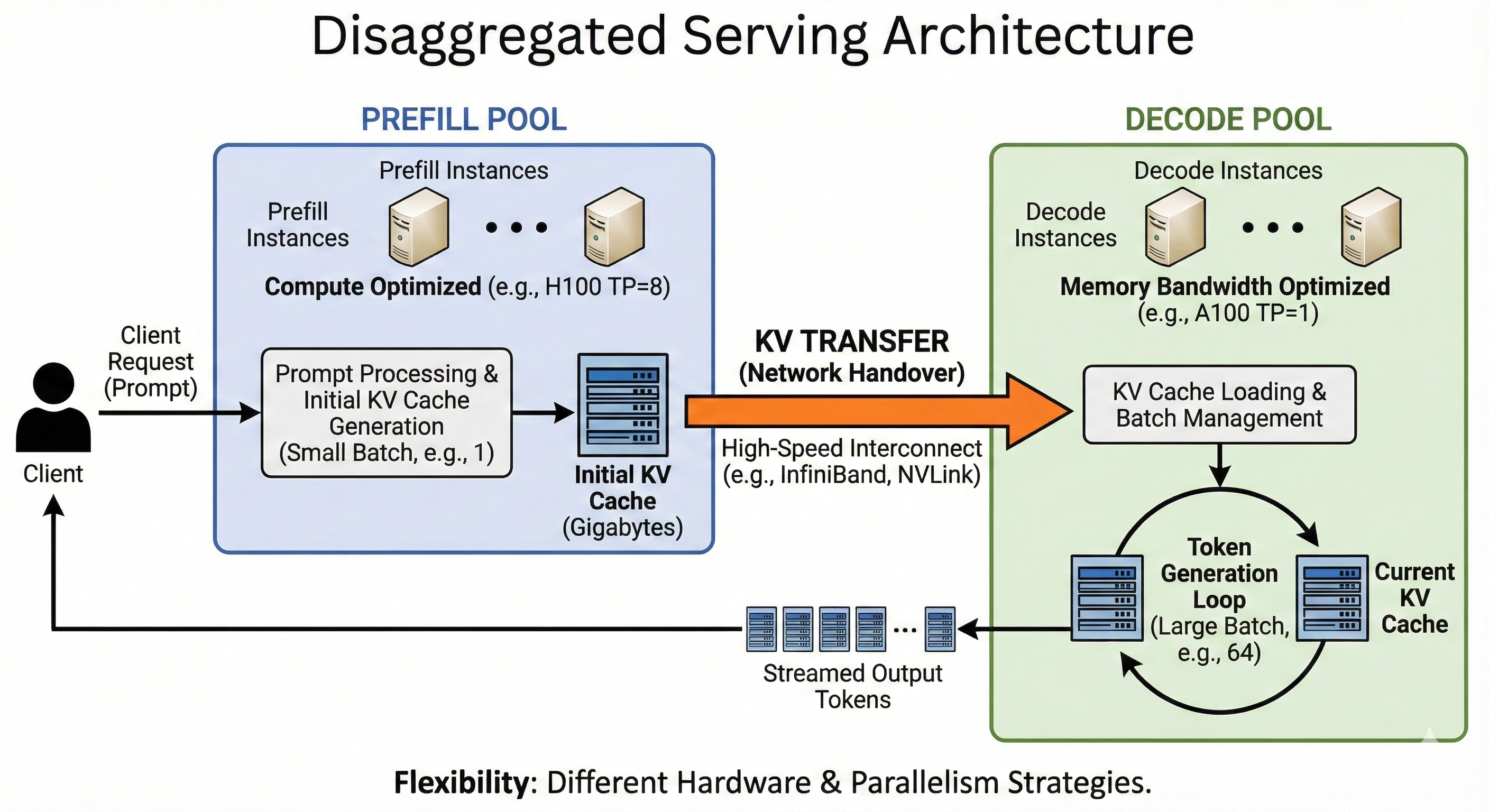
The solution is Disaggregated Serving: separating the model into two distinct pools of workers.
- Prefill Instances: Optimized for compute. They take a request, process the prompt, and generate the initial KV Cache.
- Decode Instances: Optimized for memory bandwidth. They take the initialized state and stream the rest of the tokens.
How it works
For instance, we can run a single Decode server with batch size 64, and two Prefill servers with batch size 1.
- The
Prefillserver processes a prompt and computes the initial KV Cache. - KV Transfer: This is the critical step. The Prefill server sends the computed KV Cache (which can be Gigabytes of data) over the network to the
Decodeserver. - The
Decodeserver loads this cache into its memory and adds the request to its running batch loop.
Topology and Hardware Flexibility
Because we have decoupled the phases, we are no longer forced to use the same hardware or parallelism strategies for both. We can "right-size" our infrastructure:
- Different Chip Counts (Tensor Parallelism):
- Prefill: We might shard the model across 8 GPUs (TP=8). Since we have a massive amount of computation to do, splitting the work across 8 chips divides the latency by roughly 8. This is crucial for user responsiveness.
- Decode: If we sharded the same way here, we would be waiting on network communication (All-Reduce) just to generate a few tokens. We usually favor Data Parallelism (running multiple independent copies of the model) over Tensor Parallelism. Since decoding is memory-bound, we don't need to split the compute across chips to go faster; we prefer to avoid the communication overhead of sharding.
- Different Architectures:
- Prefill: We can use compute-dense chips (e.g., NVIDIA H100) to crunch the prompt as fast as possible.
- Decode: We can use older, cheaper chips with high memory bandwidth (e.g., A100s) or even specialized inference chips, as we just need to hold the KV cache and move it to the compute units quickly.
The Trade-off: KV Transfer
There is no free lunch. The cost of this architecture is the Network Handover.
When the Prefill server finishes, the KV Cache resides in its HBM (GPU Memory). To start decoding on a different server, we must transmit this cache over the network. For long sequences, this can be Gigabytes of data.
To make this viable, we usually need high-speed interconnects (like InfiniBand or NVLink) to ensure the time spent sending the data doesn't outweigh the time saved by splitting the workload.