Pipelining
Pipelining is a model parallelism strategy used when a model is too large to fit into the memory of a single device. Instead of sharding the data, we partition the model itself.
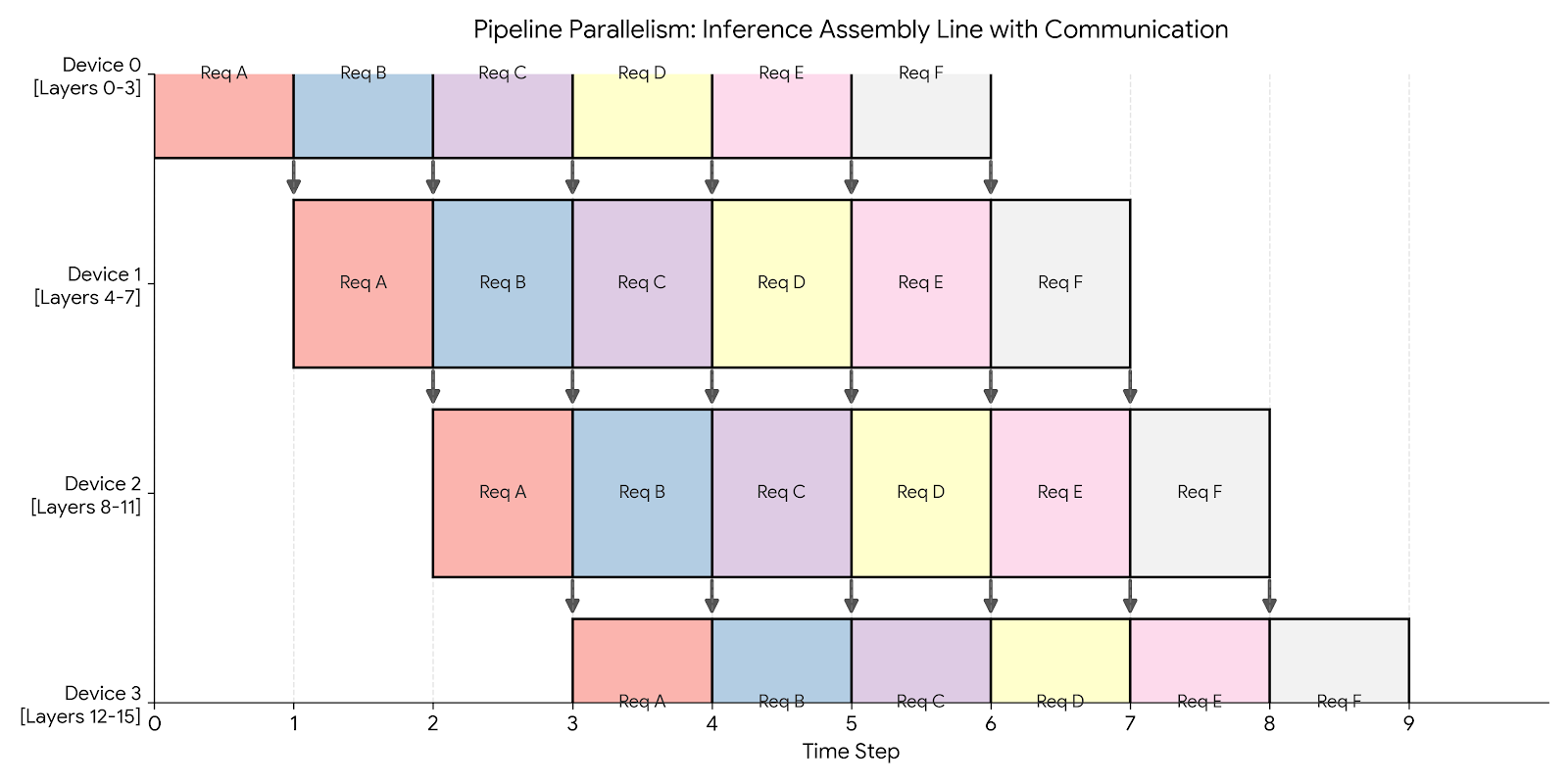
We vertically slice the model and assign a group of layers to each device. For example, if we have 4 devices and 16 layers: Device 0 holds layers 0-3, Device 1 holds layers 4-7, and so on.
Inference
During inference, Pipeline Parallelism acts like a factory assembly line.
We can achieve 100% utilization by keeping the pipeline full. As soon as Device 0 finishes processing Request A and passes it to Device 1, it immediately picks up Request B. We fully overlap communication with computation.
Code for inference only using the Fake API
We run the same model as in Fake API but with an arbitrary amount of layers. This time, we have one layer per device. Device 0 will run layer 0. Device 1 will run ReLU and layer 1, etc. So even indices will run their layers only and odd indices will run ReLU and their layer. We implement the inference_loop to handle communicating the outputs of each layer.
class PipeliningInferenceOnly(ShardedEngine):
    def __init__(self, model_dim: int, hidden_dim: int):
        if self.device_id % 2 == 0:
            self.weights = np.zeros((model_dim, hidden_dim), dtype=np.float32)
        else:
            self.weights = np.zeros((hidden_dim, model_dim), dtype=np.float32)

    def load_checkpoint(self, params: dict[str, npt.ArrayLike]) -> None:
        # Load weights into local memory
        self.weights[...] = params[f'layers_{self.device_id}/weights'][...]

    def forward(self, x: npt.ArrayLike) -> npt.ArrayLike:
        # On odd layers (which receive hidden_dim), apply ReLU first
        if self.device_id % 2 != 0:
            x = relu(x)
        return np.einsum('bd,df->bf', x, self.weights)

    def inference_loop(self, input_stream: Reader[npt.ArrayLike], output_stream: Writer[npt.ArrayLike]) -> None:
        # LOGIC FOR DEVICE 0 (The Source)
        if self.device_id == 0:
            for x in iter(input_stream):
                out = self.forward(x)
                self.send(1, out)
        # LOGIC FOR OTHER DEVICES
        else:
            while True:
                # Block until we get data from the previous device
                x = self.receive(self.device_id - 1)
                out = self.forward(x)
                # If I am the last device, write to disk/network
                if self.device_id == self.num_devices - 1:
                    output_stream.write(out)
                else:
                    self.send(self.device_id + 1, out)
Training
Training is significantly harder due to the bidirectional dependency between the forward and backward pass.
- Forward Dependency: Layer
Nneeds input from LayerN-1. - Backward Dependency: Layer
N-1needs gradients from LayerN.
This creates a wait time known as the Pipeline Bubble.
- Idle Start: Device 3 sits idle waiting for the first data to propagate through Devices 0, 1, and 2.
- Idle End: Device 0 sits idle after its backward pass, waiting for the gradients to propagate back from Device 3.
Solution: Micro-batching To minimize the bubble, we split the global batch into smaller micro-batches. By processing smaller chunks, we can pass data to the next device sooner, allowing the pipeline to fill up faster.
Pros and cons
Pipelining is optimized for throughput (requests per second) at the cost of latency (time per request). It effectively uses multiple chips to simulate a single, massive chip.
| Feature | Impact | Why? |
|---|---|---|
| Throughput | ✅ High | During inference (or well-tuned training), all devices work in parallel. |
| Communication | ✅ Low | We only send activations between devices at the boundaries (e.g., after layer 4). This is much cheaper than Tensor Parallelism. |
| Latency | ❌ High | A single request must travel sequentially through all devices. Device 4 cannot start until Device 3 finishes. |
| Memory | ✅ Efficient | Parameters are split across devices, allowing us to fit larger models. |